Summary
Which forecast does sMAPE reward? sMAPE has been criticised for its asymmetry and its behaviour near zero, but the forecast that minimises it had been found only in special cases. We show that for positive values sMAPE depends only on the ratio of actual to forecast, not on their difference: it is the hyperbolic tangent of half the absolute log error. So it scores a forecast k times too high and one k times too low the same, and is asymmetric only for equal absolute errors. Being bounded, it has a finite expected value for every distribution. Its target is a median of the actuals, each weighted by how close it is to the forecast by ratio. This is the median when the log of the actual is symmetric and unimodal; otherwise it can move to the side of the median that carries more weight. With two well-separated groups of actuals, the median becomes a local maximum. On intermittent demand the target is 0 once the share of zeros passes a threshold below one half. Otherwise sMAPE aims at a weighted median of the non-zero actuals. As the actuals spread out, expected sMAPE approaches its bound for every forecast, so forecasts become hard to tell apart, and the target moves from the median to the mode of the log. Where sMAPE and MAE both target the median, a test set's sMAPE minimiser estimates it less precisely than the sample median, increasingly so as the actuals spread out.
Highlights
- SupportS 100For and , the sMAPE term depends on and only through their ratio : . C1
- SupportS 100Let the actual be positive and take no single value with positive probability, let be its ordinary (unweighted) median, and let its expected sMAPE have a single local minimum. With the forecast at , compare the total weight of the actuals above with that of the actuals below it. (a) If the actuals above carry more weight, the sMAPE target lies above ; if those below carry more, it lies below . (b) If the two weights are equal, is a point where expected sMAPE is flat. It is then the target if, in addition, where is the density of , continuous at : this makes a strict local minimum. Without it, can be a flat point of inflection, with the target elsewhere. (c) When has a density symmetric about and unimodal, is the only target; lognormal and log-Laplace actuals are examples. C12
- SupportS 100Let the actual be positive and take no single value with positive probability. A forecast has the lowest expected sMAPE only if the actuals below and those above it carry equal total weight : So the sMAPE target is a median of the actuals weighted by , where the ordinary median gives every actual the same weight. An actual's weight is largest when it equals the forecast, is the same for and , and falls as moves away from 1 in either direction. C4
- SupportS 89Where sMAPE and MAE both target the median (log-symmetric outcomes), the sMAPE minimiser of a test set varies more than the sample median for every spread and test-set size studied: its relative efficiency is below 1 and falls as the actuals spread out, at from 0.97 to 0.03 on lognormal actuals as grows from 0.25 to 6, and from 1.00 to 0.34 on log-Laplace actuals as grows from 0.25 to 6, close to the large-sample values. C15
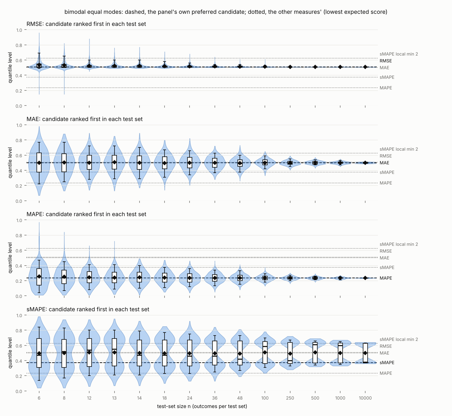
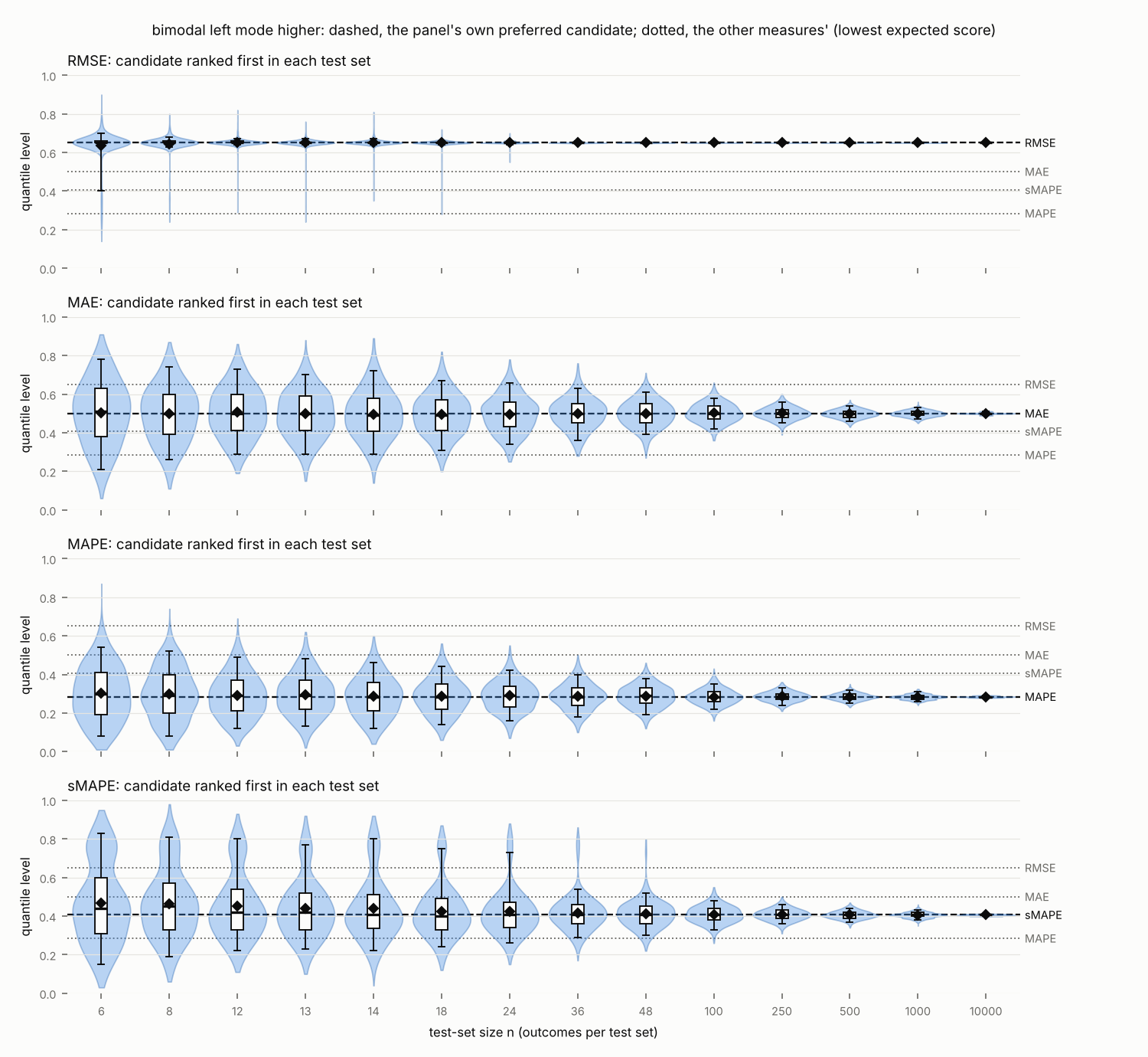
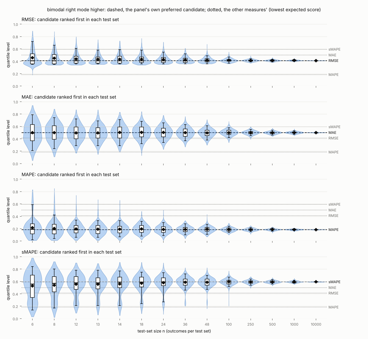
- SupportS 94Let have two modes, at and (), with the actuals concentrated near them: a mixture of a distribution near and its mirror image about , with weights and . (a) With equal weights the median lies in the gap between the two groups; when the groups are narrow enough it has a higher expected sMAPE than forecasts near either mode, and it is a local maximum of expected sMAPE; there is a minimiser on each side of the median, and these approach and as the groups narrow. (b) With unequal weights and narrow groups, the best forecast is near the mode of the larger group. C6
Context
- Extends Tofallis (2015) · from C1
- Tofallis (2015) lists the sMAPE term, |y-f|/[(|y|+|f|)/2], among Tornqvist et al.'s measures of relative change; C1 shows it depends on the actual and the forecast only through their ratio.
- Qualifies Svetunkov (2026a), C33 · from C2
- C33 says sMAPE penalises a forecast below the outcome more than one above it. That holds for two forecasts the same absolute distance away (C2 b); a forecast k times too low and one k times too high score the same (C2 a).
- Refines Goodwin and Lawton (1999) · from C2
- Goodwin and Lawton (1999) showed that sMAPE is asymmetric: for the same absolute error it scores a forecast above the actual better than one below. C2 proves this (b) and shows that by ratio sMAPE is symmetric (a).
- Refines Hyndman and Koehler (2006) · from C2
- Hyndman and Koehler (2006) note that for the same actual sMAPE penalises low forecasts more heavily than high ones; C2 shows this holds for equal absolute errors and not for equal ratios.
- Refines Hewamalage et al. (2023) · from C2
- Hewamalage et al. (2023) note that sMAPE penalises underestimates more than overestimates for the same actual; C2 shows this holds for equal absolute errors and not for equal ratios.
- Refines Chen et al. (2017) · from C2
- Chen et al. (2017) show a heavier penalty on a forecast 10% under the actual than on one 10% over; C2 shows that forecasts the same factor too high and too low score the same.
- Extends Tofallis (2015) · from C3
- Tofallis (2015) relates sMAPE to the log accuracy ratio among relative measures; C3 shows the sMAPE term is exactly the hyperbolic tangent of half the absolute log ratio.
- Explains Svetunkov (2026b), C5 · from C4
- C5 found sMAPE's preferred candidate close to the median on other distributions; C4 shows why: the target is a weighted median, on the side of the median that carries more weight (C12).
- Addresses Tofallis (2015) · from C4
- Tofallis (2015) states that minimising sMAPE does not produce an established measure of location; C4 identifies the target as a median weighted by y/(y+f)^2.
- Qualifies Hewamalage et al. (2023) · from C4
- Hewamalage et al. (2023) say sMAPE may tend towards selecting a slightly overestimating model; C4 shows the target is a weighted median, which lies on the side of the median that carries more weight, above or below it (C12).
- Replicates Anderson (1955) · from C5
- C5 is an elementary case of Anderson's theorem on symmetric unimodal densities, proved here directly for the expected sMAPE.
- Refines Svetunkov (2026b), C6 · from C7
- C6 found sMAPE preferring zero on counts with more than half zeros; C7 gives the exact threshold, which is below one half whenever the positive outcomes vary.
- Extends Kolassa (2026) · from C7
- Kolassa (2026) shows that sMAPE elicits a zero forecast for sufficiently intermittent actuals; C7 gives the share of zeros at which it does, which is below one half.
- Extends Hewamalage et al. (2023) · from C9
- Hewamalage et al. (2023) note that sMAPE is bounded by 200; C9 adds that its expected value is therefore finite for every distribution and that a best forecast exists.
- Supports Svetunkov (2026a), C6 · from C10
- C6 recommends against sMAPE for point forecasts; C10 shows that on widely spread actuals every forecast scores close to the worst value and the target moves to the mode of ln y.
- Supports Kolassa (2026) · from C10
- Kolassa (2026) concludes that sMAPE should not be used; C10 shows that on widely spread actuals every forecast scores close to the worst value.
- Explains Svetunkov (2026b), C5 · from C12
- C5 found by simulation that sMAPE prefers the median on lognormal and log-Laplace outcomes; C12 proves it for every symmetric unimodal ln y.
- Supports Svetunkov (2026b), C11 · from C15
- C11 found sMAPE's choices in short test sets spreading more than MAE's; C15 measures the loss of precision for test sets of 6 to 10000 outcomes.
- Supports Svetunkov (2026a), C6 · from C15
- C6 recommends against sMAPE for point forecasts; C15 shows that even where it targets the median it estimates it less precisely than the sample median.
- Supports Kolassa (2026) · from C15
- Kolassa (2026) concludes that sMAPE should not be used; C15 shows that even where it targets the median it estimates it less precisely than the sample median.
- Extends Hewamalage et al. (2021) · from C17
- Hewamalage, Bergmeir and Bandara (2021) evaluate forecasts with the Suilin loss, Suilin's modification of sMAPE for series with values near zero; C17 shows that it keeps sMAPE's behaviour away from zero and becomes an absolute error near zero.
- Supports Svetunkov (2026a), C6 · from C18
- C6 recommends against sMAPE for point forecasts; C18 shows that on widely spread actuals a test set tells two forecasts apart less and less well under sMAPE.
- Supports Kolassa (2026) · from C18
- Kolassa (2026) concludes that sMAPE should not be used; C18 shows that on widely spread actuals a test set tells two forecasts apart less and less well under sMAPE.
- Extends Kolassa (2026) · from C20
- Kolassa (2026, Proposition 3) shows that the minimisers of expected msMAPE on counts are integers; C20 shows where the msMAPE term equals the sMAPE term and that it removes the jump at the zero forecast.
- Extends Smyl (2025) · from C20
- Smyl (2025) proposed msMAPE, the sparse-proof sMAPE, as Kolassa (2026) reports; Smyl's article was not read. C20 states properties of its term as Kolassa (2026, Definition 4) defines it.
Definitions
Methods 4
D16 selection design: For each outcome distribution: derive the candidate forecasts and their expected scores; then, for each test-set size , draw test sets of independent outcomes, score every candidate by every measure on each test set, and count the candidate with the lowest score as the measure's choice (a tie of candidates counts each; a test set in which every candidate scores infinite chooses none).
D17 efficiency design: For each outcome distribution and test-set size : draw test sets of independent outcomes; in each, compute the sample median and the exact sMAPE minimiser (an outcome of the test set, since the test set's sMAPE is concave in between consecutive outcomes); over test sets, compare the variances of their logarithms.
D18 flatness design: For families whose spread of grows from 0.1 to 10: derive the sMAPE target, the expected sMAPE of forecasts at fixed quantile levels and the large-spread approximation of C10; on test sets, count how often each measure scores the target lower than a forecast away from it, and where the test set's sMAPE minimiser falls.
D31 formula checks: Numerical checks of the formulas of the formal claims (claimset-code/smape-target/check_formulas.py, seed 6; check_jump.py for C11): identities and inequalities on 200000 random pairs, derivatives against finite differences, minimisers, balances and thresholds against quadrature and bisection on every setting of the selection design, and the large-spread expansion against its bound. For the claims new or reworded in version 3 (C3, C4, C12, C17 to C20): check_v3.py (seed 8), check_h39.py and check_corrected.py (seed 8), in the same way.
Variables and measures 15
D2 sMAPE: Symmetric mean absolute percentage error of a point forecast over a test set of actuals : , where a term with counts as 0. Introduced as the symmetric MAPE by Makridakis (1993), whose denominator had no absolute values; for positive actuals and forecasts the two agree. Source: Makridakis (1993).
D1 sMAPE term: The contribution of one actual and one point forecast to sMAPE: , between 0 and 1, with when (including , where the fraction is ).
D3 expected sMAPE: The expected sMAPE of a fixed forecast under the distribution of the actual : , where is the expectation over the random actual . Computed from the distribution (by integration or exact sums), never from a sample.
D4 log error: For a positive actual and a positive forecast , .
D5 weight: For a positive actual and a positive forecast , : how much the actual pulls the forecast that minimises expected sMAPE, since the derivative of in is . Largest at , the same for and .
D10 RMSE: Root mean squared error of a point forecast over a test set of actuals : .
D11 MAE: Mean absolute error of a point forecast over a test set of actuals : .
D12 MAPE: Mean absolute percentage error of a point forecast over a test set of actuals : ; infinite when an actual is zero.
D19 log-MAE: 100 times the mean absolute error of as a forecast of : . Unbounded; sMAPE's small-error limit (C3); minimised by the median.
D28 Suilin term: The contribution of one actual and one forecast to the Suilin loss: the Suilin loss is 200 times its mean over a test set. It replaces the denominator of the sMAPE term. Proposed by Suilin (2017) in code for a Kaggle competition, as a smoothed variant of sMAPE; defined in print by Hewamalage, Bergmeir and Bandara (2021, Eq. 15), who write the constant as and the factor 2 into the measure differently (a constant factor changes no property here). Hewamalage, Ackermann and Bergmeir (2023) call it msMAPE; Smyl (2025) gives that name to a different measure, so this study follows Kolassa (2026) and calls it the Suilin loss. Version 2 of this paper called it msMAPE. Source: Hewamalage et al. (2021).
D33 msMAPE term: The contribution of one actual and one forecast to the sparse-proof sMAPE (msMAPE) of Smyl (2025), as Kolassa (2026, Definition 4) states it, for a small constant (Kolassa writes it , which is the median here): which is 0 when ; msMAPE is 200 times its mean over a test set (Kolassa writes the factor 2 into the term). It replaces the actual in the denominator of the sMAPE term by when the actual is below . Source: Kolassa (2026).
D8 sMAPE minimiser of a test set: The forecast that minimises the sMAPE of one test set , , found numerically (the sample counterpart of the sMAPE target).
D9 relative efficiency: For a test-set size and an outcome distribution where sMAPE and MAE both target the median: over test sets, where is the sample median (the MAE minimiser) and the sMAPE minimiser of the same test set. Above 1, sMAPE's minimiser varies less; below 1, MAE's does.
D20 ranking agreement: For one distribution, one measure, a test-set size , the measure's target and a forecast at another quantile level: the probability that a test set of outcomes gives the target the strictly lower score (ties count as disagreement); 0.5 is a coin toss.
D32 signal-to-noise ratio of a comparison: For a measure with term , two forecasts and and a distribution of the actual : , where is the difference of the two forecasts' scores on one actual. Over a test set of independent actuals the mean of is times this many of its standard errors from zero: the larger the ratio, the smaller the test set that tells the two forecasts apart.
Populations 9
D21 inverse Gaussian outcomes: Inverse Gaussian outcomes with mean 100 and shape 1000, 200, 100, 50, 20 or 10 (coefficient of variation 0.32 to 3.16): positive, skewed right, every moment and finite.
D22 log-skewed outcomes: with , : with standard deviation (0.5 or 1; sd in the settings' names) and skewness (-2, -1, -0.5, +0.5, +1, +2), and the lognormal of the same (skewness 0). Some have infinite moments: infinite (, skewness +2), infinite (, skewness +2; , skewness +1), infinite (, skewness -2).
D23 bimodal outcomes: , normal with mean (probability ) or , standard deviation 0.25; (equal modes), 0.65 (left mode higher), 0.35 (right mode higher).
D24 outcomes straddling zero: Normal outcomes with standard deviation 1 and mean 0, 0.5 or 1: 50%, 31% and 16% negative; infinite.
D25 zero-inflated outcomes: Lognormal outcomes (median 100, 0.5 or 1) replaced by 0 with probability : 0.25, 0.42, 0.47, 0.6 for and 0.25, 0.37, 0.42, 0.6 for , on both sides of the zero threshold of C7 (0.4469 and 0.3940).
D26 log-symmetric outcomes: Lognormal outcomes with , and log-Laplace outcomes with scale , each 0.25, 0.5, 1, 1.5, 2, 3, 4 or 6, median 100: symmetric and strictly unimodal, so that sMAPE and MAE both target the median (C5).
D27 widening outcomes: with standard normal (lognormal), standard Gumbel (log-Gumbel right, skewed right) or minus standard Gumbel (log-Gumbel left), for = 0.1, 0.25, 0.5, 1, 1.5, 2, 3, 4, 6 and 10.
D30 Poisson counts: Poisson outcomes with means 0.3, 0.5, 1, 1.5, 3 and 10: counts whose share of zeros falls from 0.74 to almost 0.
D35 intermittent demand settings: Demand with many zeros. Counts: Poisson with means 0.1, 0.3, 0.5, 0.7, 1, 1.5 and 3 (share of zeros from 0.90 to 0.05) and, overdispersed, negative binomial with size 0.5 and means 0.5, 1 and 2 (share of zeros 0.71, 0.58 and 0.45). Non-integer demand: lognormal demand sizes (median 1, ) replaced by 0 with probability 0.2, 0.4, 0.6 or 0.8.
Concepts 7
D6 sMAPE target: The value or values of that minimise expected sMAPE for a given distribution of the actual , : the functional sMAPE rewards. It may be a single value or several.
D7 quantile profile: For an outcome distribution with quantile function and a forecast , the pull of the outcome at each quantile level , on ; the minimiser's quantile level balances its integrals below and above.
D29 Suilin target: The value or values of that minimise the expected Suilin term for a given distribution of the actual: the functional the Suilin loss rewards, as the sMAPE target is the one sMAPE rewards.
D34 msMAPE target: The value or values of that minimise the expected msMAPE term for a given distribution of the actual and a given constant : the functional msMAPE rewards, as the sMAPE target is the one sMAPE rewards.
D13 candidate forecast: A point forecast fixed from the outcome distribution before any test set is drawn and the same for every test set: a quantile at a level from 0.01 to 0.99, the mean, the forecast 0, the log-mode, the minimiser of expected MAPE, or a local minimiser of expected sMAPE. It is never estimated from a sample.
D14 preferred candidate: Of the candidate forecasts for one distribution, the one a measure gives the lowest expected score, or, where every expected score is infinite but their differences are finite, the one the differences rank first (C8); none where no forecast is ranked first.
D15 derived value: A value computed from the outcome distribution itself by numerical integration of its density (Gauss-Legendre quadrature and a convolution on a grid of 524288 points of ), never from a sample: the expected scores, the local minima of expected sMAPE, the formulas of the hypotheses.
Principal claims
For and , the sMAPE term depends on and only through their ratio : .
Proof: E18 · Data: E1 · Extends: Tofallis (2015) · Verification: checked by an agent · Planned: lab plan PL9, planned 17 November 2026 · Outcome: judged by the writer
For and , the sMAPE term is (log error ). (a) It is 0 when , strictly increasing and concave in , and bounded by 1, which it approaches as grows. (b) ; so when all log errors are small, sMAPE is about 100 times the mean absolute error of as a forecast of (log-MAE). (c) The log-MAE of a test set is minimised by its median; sMAPE is then minimised near the median, not in general at it. For positive actuals with a median , a forecast that minimises their sMAPE satisfies its mean absolute log error exceeds the smallest possible by at most a twelfth of its mean cubed absolute log error. The minimiser is the median itself only under further conditions on the distribution of the actuals.
Proof: E20 · Data: E31 · Uses: C1 · Extends: Tofallis (2015) · Verification: checked by an agent · Planned: lab plan PL12, planned 18 November 2026 · Outcome: judged by the writer
Let the actual be positive and take no single value with positive probability. A forecast has the lowest expected sMAPE only if the actuals below and those above it carry equal total weight : So the sMAPE target is a median of the actuals weighted by , where the ordinary median gives every actual the same weight. An actual's weight is largest when it equals the forecast, is the same for and , and falls as moves away from 1 in either direction.
Proof: E22 · Data: E31 · Uses: C9 · Explains: Svetunkov (2026b), C5 · Addresses: Tofallis (2015) · Qualifies: Hewamalage et al. (2023) · Qualifies: C2 · Verification: checked by an agent · Planned: lab plan PL12, planned 18 November 2026 · Outcome: judged by the writer
Let have two modes, at and (), with the actuals concentrated near them: a mixture of a distribution near and its mirror image about , with weights and . (a) With equal weights the median lies in the gap between the two groups; when the groups are narrow enough it has a higher expected sMAPE than forecasts near either mode, and it is a local maximum of expected sMAPE; there is a minimiser on each side of the median, and these approach and as the groups narrow. (b) With unequal weights and narrow groups, the best forecast is near the mode of the larger group.
Proof: E24 · Data: E1 · Uses: C3, C9, C12 · Verification: checked by an agent · Planned: lab plan PL9, planned 17 November 2026 · Outcome: judged by the writer
A forecast of the opposite sign to the actual, a zero forecast of a non-zero actual, and a non-zero forecast of a zero actual all give the sMAPE term its largest value, 1. Let the actual be 0 with probability and otherwise positive, and the lowest expected a positive forecast reaches on the positive actuals. The forecast 0 is the sMAPE target when , and a positive forecast does when the inequality is reversed; the threshold is below whenever .
Proof: E25 · Data: E1 · Uses: C9 · Refines: Svetunkov (2026b), C6 · Extends: Kolassa (2026) · Verification: checked by an agent · Planned: lab plan PL9, planned 17 November 2026 · Outcome: judged by the writer
For actuals and forecasts of any sign, . So the expected sMAPE of every forecast is finite, between 0 and 200, whatever the distribution of the actuals and without any moment of it being finite (unlike RMSE, MAE and MAPE, C8). For a positive random actual , at least one forecast has the lowest expected sMAPE.
Proof: E21 · Data: E1 · Uses: C3 · Extends: Hewamalage et al. (2023) · Verification: checked by an agent · Planned: lab plan PL9, planned 17 November 2026 · Outcome: judged by the writer
Let , where has a fixed density with bounded continuous first and second derivatives, and write a forecast as (its quantile level, the probability that , does not depend on ). As grows, uniformly in . (a) The expected sMAPE of every forecast tends to its bound 200, and the difference between forecasts at two fixed quantile levels shrinks like . (b) When has a single highest point , the quantile level of the sMAPE target tends to that of , the mode of , which differs from 1/2 when the mode of is not its median. (c) As , when has a unique median and a finite , the quantile level of the target tends to 1/2: sMAPE targets the median for narrow distributions and the mode of for wide ones.
Proof: E28 · Data: E1 · Uses: C3 · Supports: Svetunkov (2026a), C6 · Supports: Kolassa (2026) · Verification: checked by an agent · Planned: lab plan PL9, planned 17 November 2026 · Outcome: judged by the writer
Let the actual be positive and take no single value with positive probability, let be its ordinary (unweighted) median, and let its expected sMAPE have a single local minimum. With the forecast at , compare the total weight of the actuals above with that of the actuals below it. (a) If the actuals above carry more weight, the sMAPE target lies above ; if those below carry more, it lies below . (b) If the two weights are equal, is a point where expected sMAPE is flat. It is then the target if, in addition, where is the density of , continuous at : this makes a strict local minimum. Without it, can be a flat point of inflection, with the target elsewhere. (c) When has a density symmetric about and unimodal, is the only target; lognormal and log-Laplace actuals are examples.
Proof: E29 · Data: E31 · Uses: C3, C4, C5, C9 · Explains: Svetunkov (2026b), C5 · Verification: checked by an agent · Planned: lab plan PL12, planned 18 November 2026 · Outcome: judged by the writer
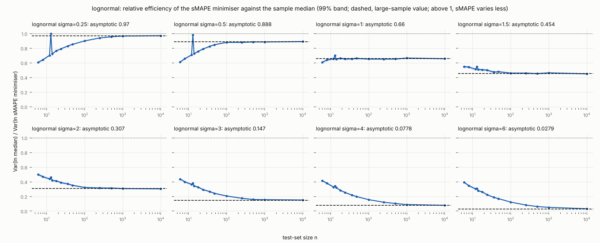
Where sMAPE and MAE both target the median (log-symmetric outcomes), the sMAPE minimiser of a test set varies more than the sample median for every spread and test-set size studied: its relative efficiency is below 1 and falls as the actuals spread out, at from 0.97 to 0.03 on lognormal actuals as grows from 0.25 to 6, and from 1.00 to 0.34 on log-Laplace actuals as grows from 0.25 to 6, close to the large-sample values.
Scope: data: test sets of independent draws from known distributions; conditions: lognormal and log-Laplace outcomes, spread 0.25 to 6, test sets of 6 to 10000 outcomes · Data: E15 (T1.r1, T1.r8, T1.r9, T1.r16) · Limitations: L2 · Supports: Svetunkov (2026b), C11 · Supports: Svetunkov (2026a), C6 · Supports: Kolassa (2026) · Qualifies: C12 · Planned: lab plan PL2, planned 16 November 2026 · Weaknesses: the code changed after the plan
The Suilin term has the properties of the sMAPE term except near zero. (a) Where , the sMAPE term shrunk by a factor between and 1 that tends to 1 as grows. So for actuals and forecasts large compared with , is close to , though no longer exactly a function of the ratio ; on counts, where every actual is 0 or at least 1, this case covers every pair except a zero actual with . (b) Where , , an absolute error: a zero forecast of a zero actual scores 0, and a forecast with of a zero actual scores , where the sMAPE term gives every non-zero forecast of a zero actual its largest value, 1. (c) everywhere, so the expected Suilin loss of every forecast is finite.
Proof: E30 · Data: E31 · Extends: Hewamalage et al. (2021) · Verification: checked by an agent · Planned: lab plan PL12, planned 18 November 2026 · Outcome: judged by the writer
Let , where has a fixed density with bounded continuous first and second derivatives and distribution function , and compare two forecasts at fixed quantile levels, and with , by their signal-to-noise ratio of a comparison. (a) For the sMAPE term, as grows, So when the ratio is it falls to zero like , and the size of the test set that keeps the mean difference a given number of standard errors from zero grows in proportion to . (b) For the absolute log error (log-MAE), , so the ratio, wherever , does not depend on . (c) For the absolute error (MAE), as grows the ratio tends to when ; the limit is positive unless the higher forecast is the median. (d) For the squared error (RMSE), when is finite the ratio is ; for lognormal actuals, times the ratio tends to 1 as grows. For widely spread actuals, then: the absolute log error keeps its power to tell two forecasts apart wherever its ratio is defined. The absolute error keeps it when and the higher forecast is not the median. sMAPE loses it at the rate when . It loses it faster, with a ratio of at most order , when . The squared error on lognormal actuals loses it faster than any power of .
Proof: E35 · Data: E32 · Uses: C3, C10 · Supports: Svetunkov (2026a), C6 · Supports: Kolassa (2026) · Refines: C10 · Verification: checked by an agent · Planned: lab plan PL17, planned 18 November 2026 · Outcome: judged by the writer
Let have a density that is symmetric about , unimodal ( whenever , strictly on a set of positive probability) and continuous at . Write , and . (a) . (b) Over test sets of independent actuals, the sMAPE minimiser of a test set (a forecast with the lowest sMAPE of the test set) tends to in probability, and is asymptotically normal with mean 0 and variance ; for the sample median the variance is . The ratio of these two limiting variances, the asymptotic relative efficiency of the sMAPE minimiser to the sample median, is that the relative efficiency of finite test sets tends to it is not shown here, since the variances of finite test sets need not tend to those of the limits. (c) For lognormal actuals with standard deviation of : as and as . For log-Laplace actuals with scale of : as and as . So on both families the sMAPE minimiser is asymptotically as precise as the sample median for narrow distributions and asymptotically loses all of its precision relative to it as the actuals spread out.
Proof: E36 · Data: E33 · Cited: Vaart (1998), Theorems 5.7 and 5.23 · Uses: C3, C5, C12 · Explains: C15 · Verification: checked by an agent · Planned: lab plan PL15, planned 18 November 2026 · Outcome: judged by the writer
The msMAPE term is the sMAPE term except for actuals below . For , and : (a) where , ; so when every actual is at least , msMAPE is sMAPE and has the same target. (b) Where , : for a zero actual it is , which is 0 at and rises towards 1 as grows, where the sMAPE term is 1 for every . (c) , with where ; and for every , is continuous in at , so the expected msMAPE term has no jump at the zero forecast, where the expected sMAPE term jumps when zero actuals have positive probability. (d) On counts with , differs from only for zero actuals.
Proof: E37 · Data: E31 · Extends: Kolassa (2026) · Extends: Smyl (2025) · Verification: checked by an agent · Planned: lab plan PL12, planned 18 November 2026 · Outcome: judged by the writer
Supporting claims
For and : (a) replacing by leaves the sMAPE term unchanged, so a forecast times too high () and one times too low () score the same; (b) of two forecasts the same absolute distance from (), the higher one scores better:
Proof: E19 · Data: E1 · Uses: C1 · Qualifies: Svetunkov (2026a), C33 · Refines: Goodwin and Lawton (1999) · Refines: Hyndman and Koehler (2006) · Refines: Hewamalage et al. (2023) · Refines: Chen et al. (2017) · Verification: checked by an agent · Planned: lab plan PL9, planned 17 November 2026 · Outcome: judged by the writer
Let have a density symmetric about , , and unimodal: whenever , strictly on a set of positive probability. Then the median of is the only sMAPE target.
Proof: E23 · Data: E1 · Uses: C3 · Replicates: Anderson (1955) · Verification: checked by an agent · Planned: lab plan PL9, planned 17 November 2026 · Outcome: judged by the writer · Used by: C12, C19
For a positive random actual : (a) RMSE: is finite exactly when is; when is infinite but finite, every difference between two forecasts and , is finite and the mean is preferred to every other forecast; when is infinite no forecast is preferred to all others. (b) MAE: is finite exactly when is; otherwise differences are finite and a median is still preferred. (c) MAPE: when is finite, the expected MAPE is finite and minimised by a median of the actuals weighted by ; when is infinite, every positive forecast has infinite expected MAPE while the forecast 0 has MAPE 100, so MAPE targets 0; when is 0 with positive probability, MAPE is infinite or undefined for every forecast and targets nothing.
Proof: E27 · Data: E1 · Verification: checked by an agent · Planned: lab plan PL9, planned 17 November 2026 · Outcome: judged by the writer
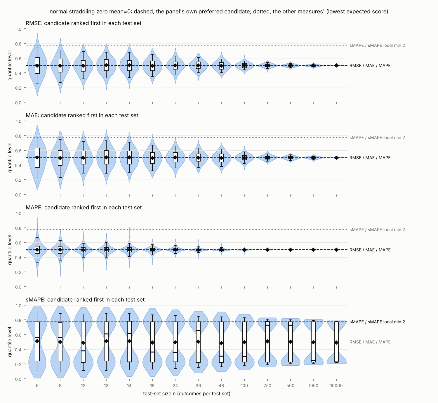
Let the actuals be , where is symmetric about 0 and its density decreases away from 0 (for example, normal). If , every forecast with the lowest expected sMAPE is positive; if , every one is negative. These forecasts stay away from 0 as approaches 0. So as moves from slightly below 0 to slightly above, the sMAPE target jumps from a negative forecast to a positive one.
Proof: E26 · Data: E11 · Uses: C7, C9 · Verification: checked by an agent · Planned: lab plan PL7, planned 16 November 2026 · Outcome: judged by the writer
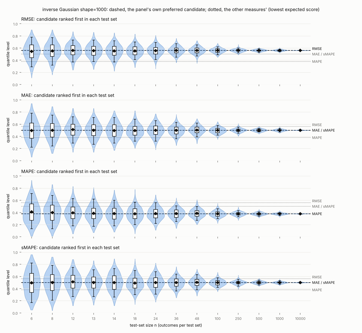
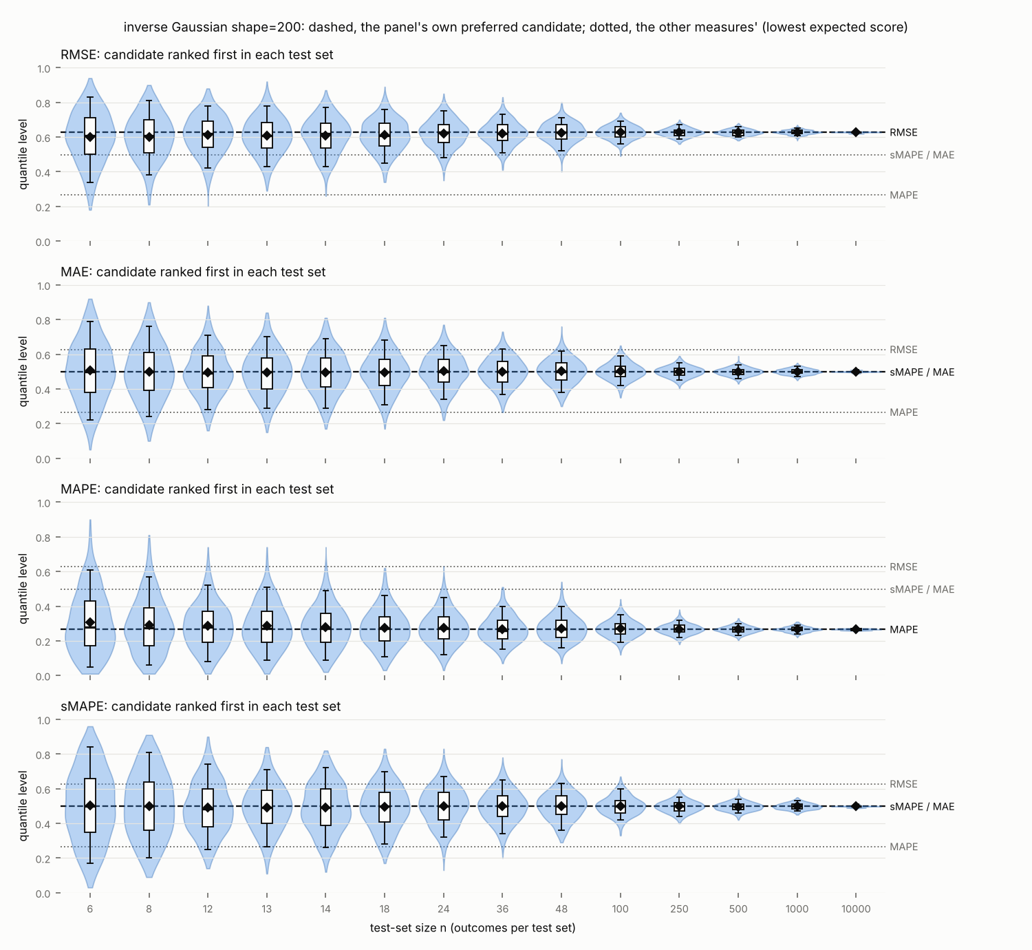
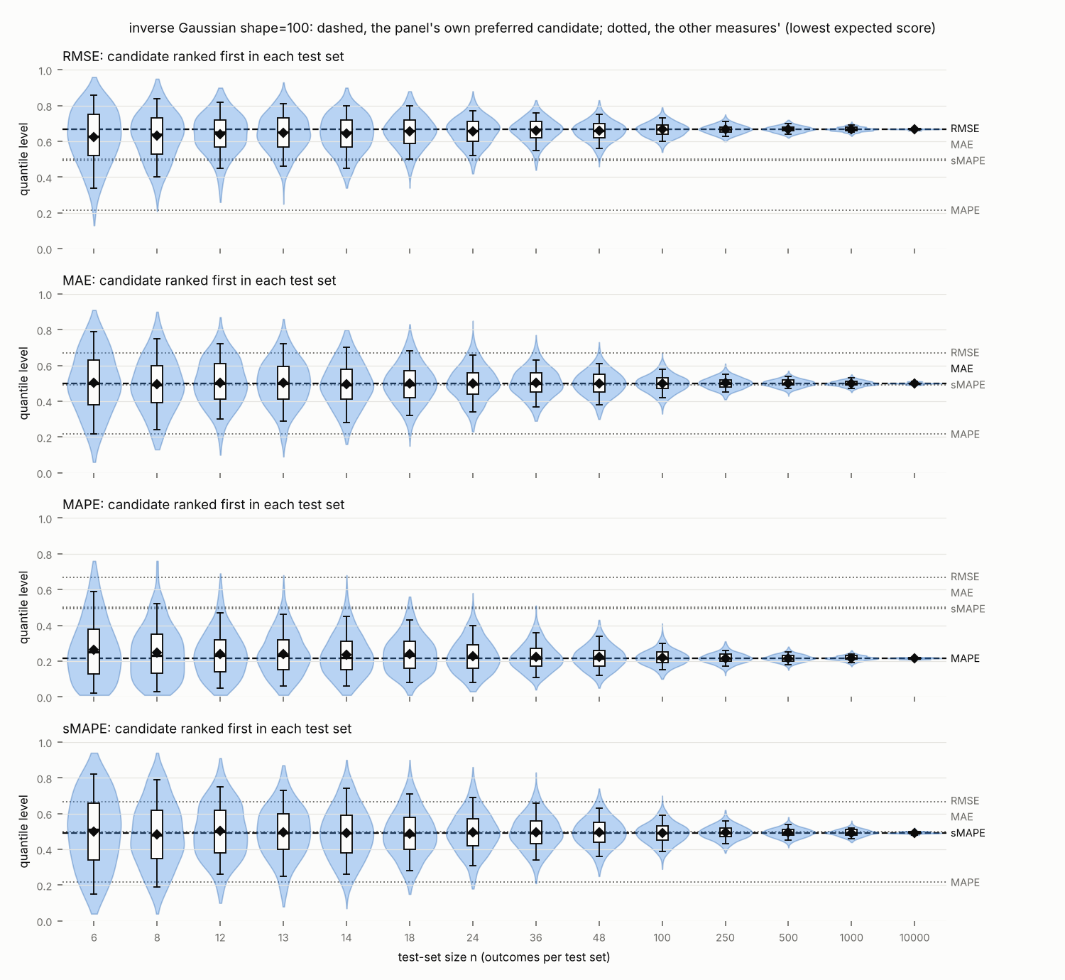
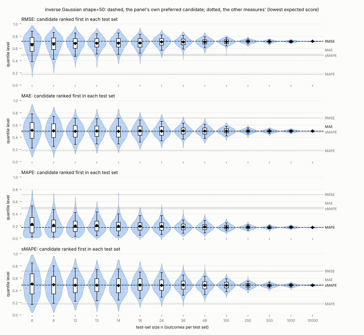
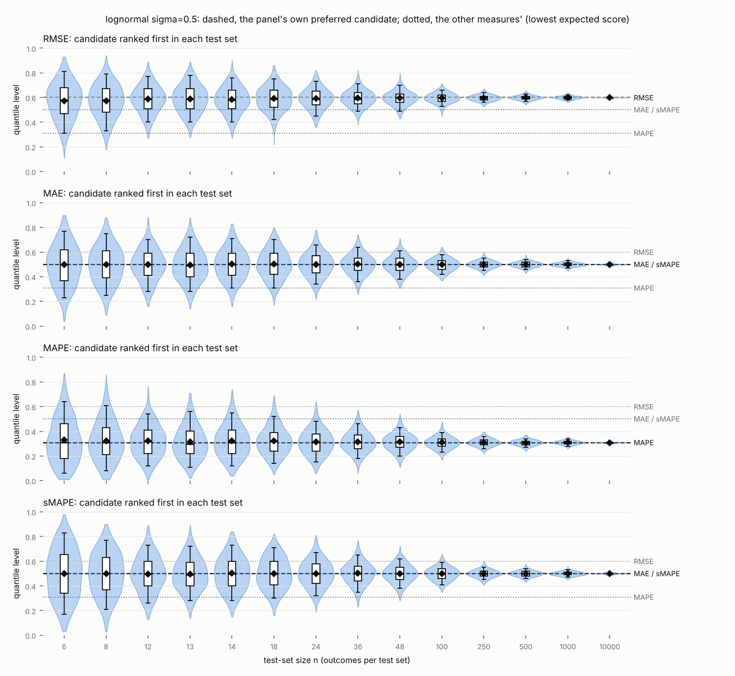
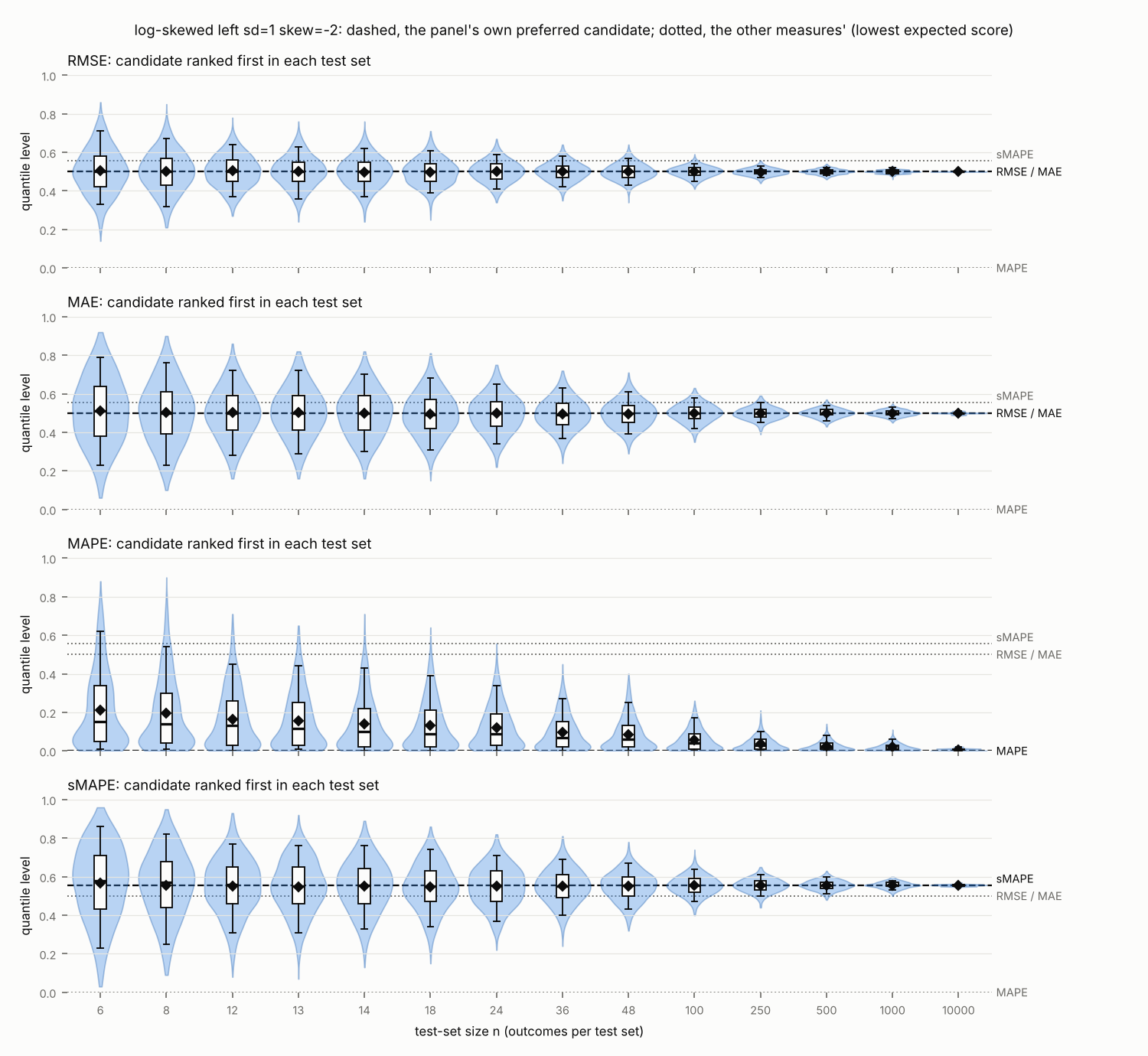
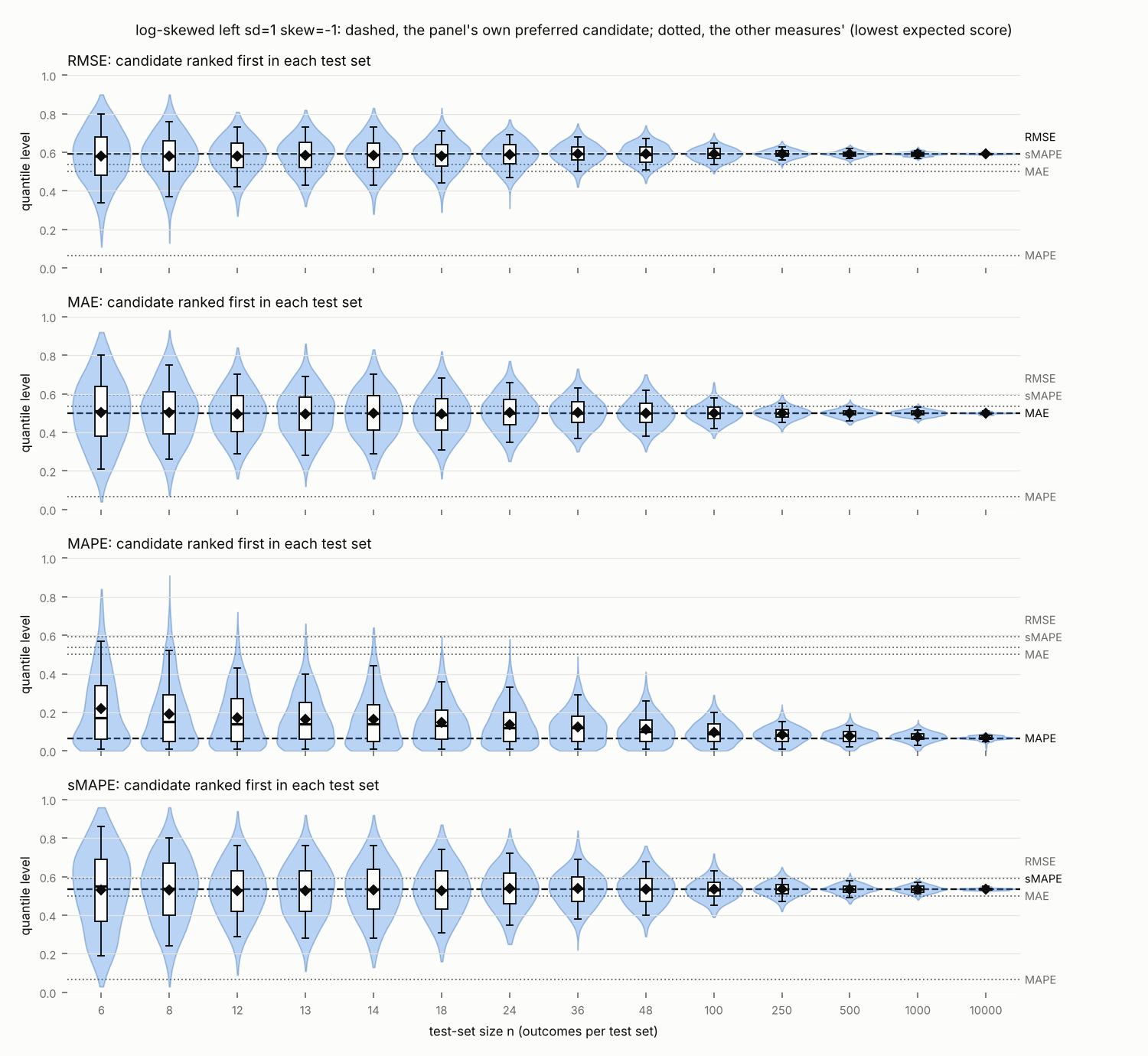
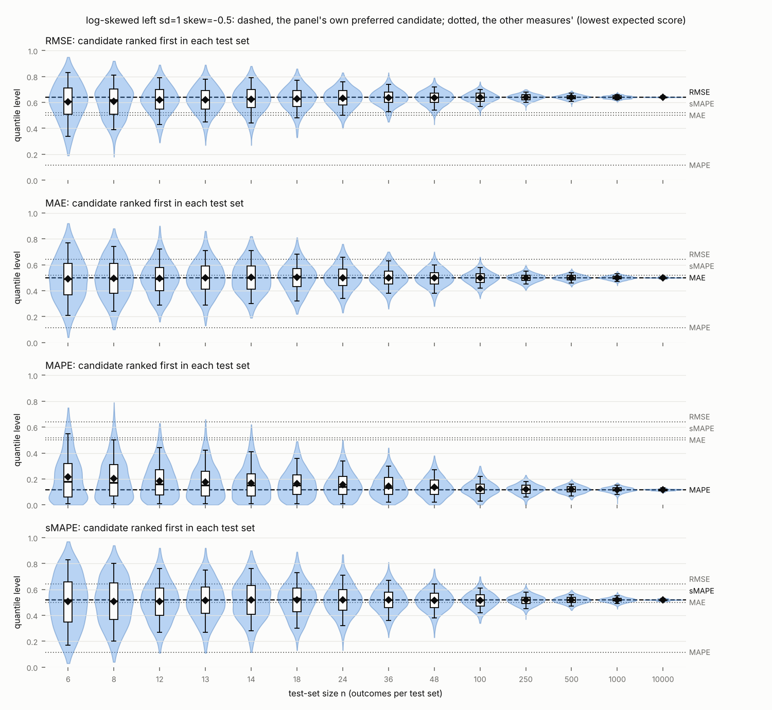
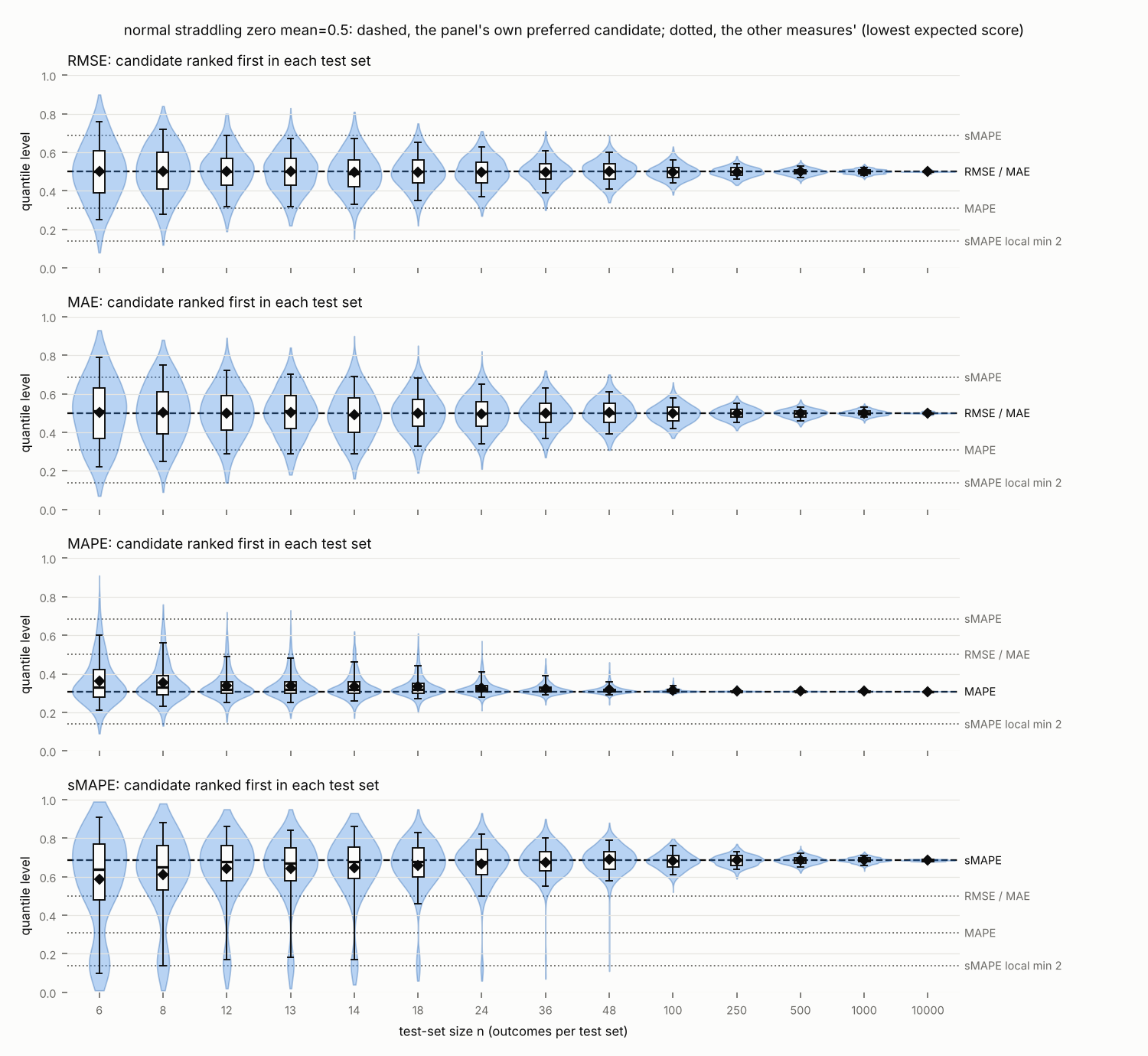
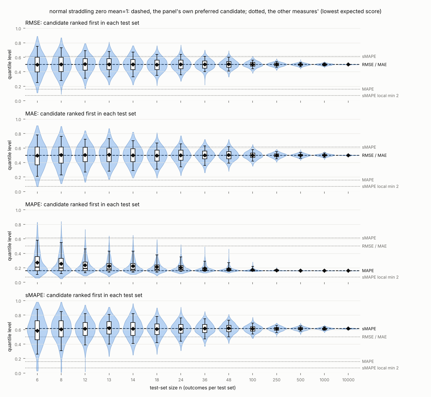
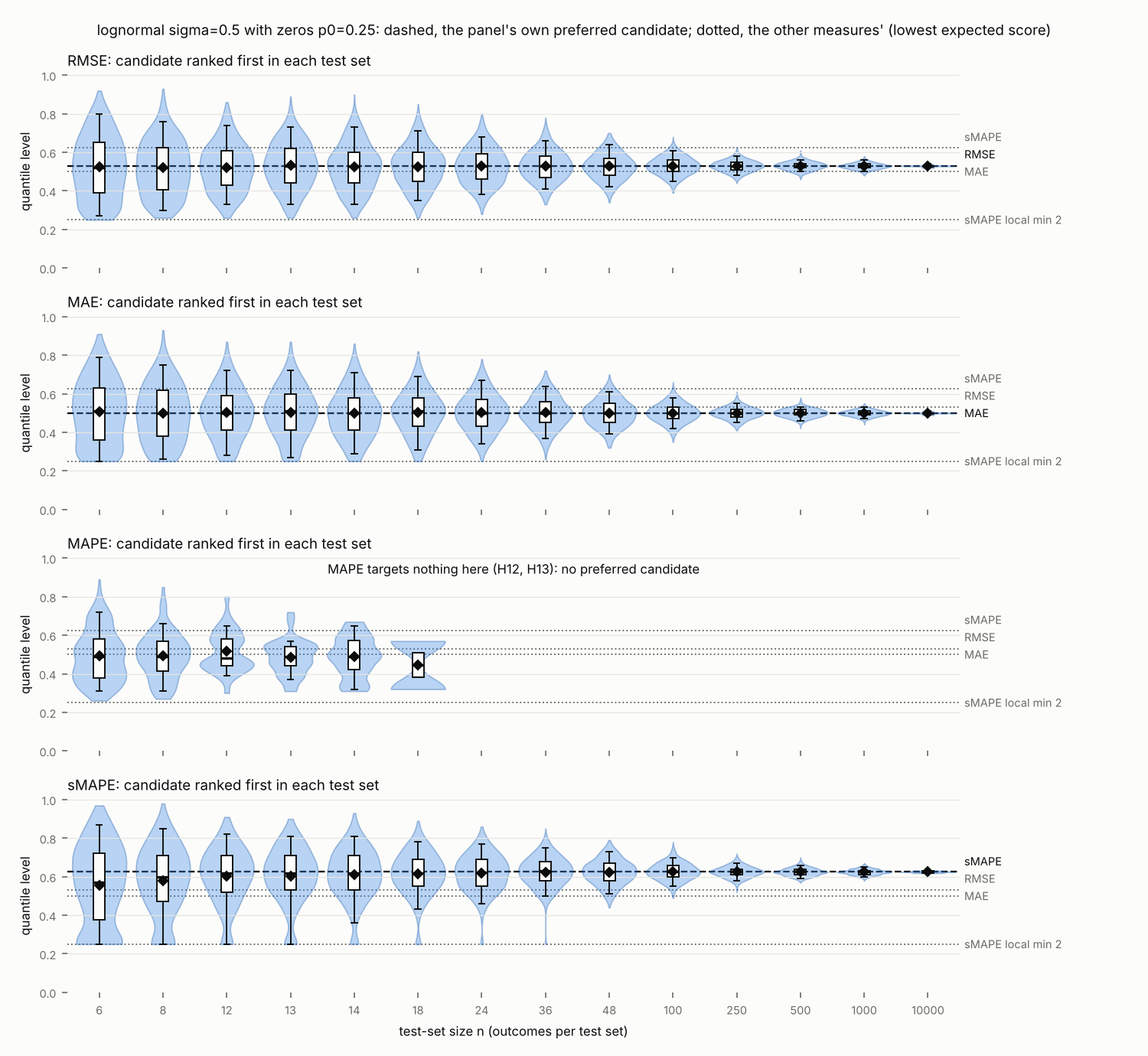
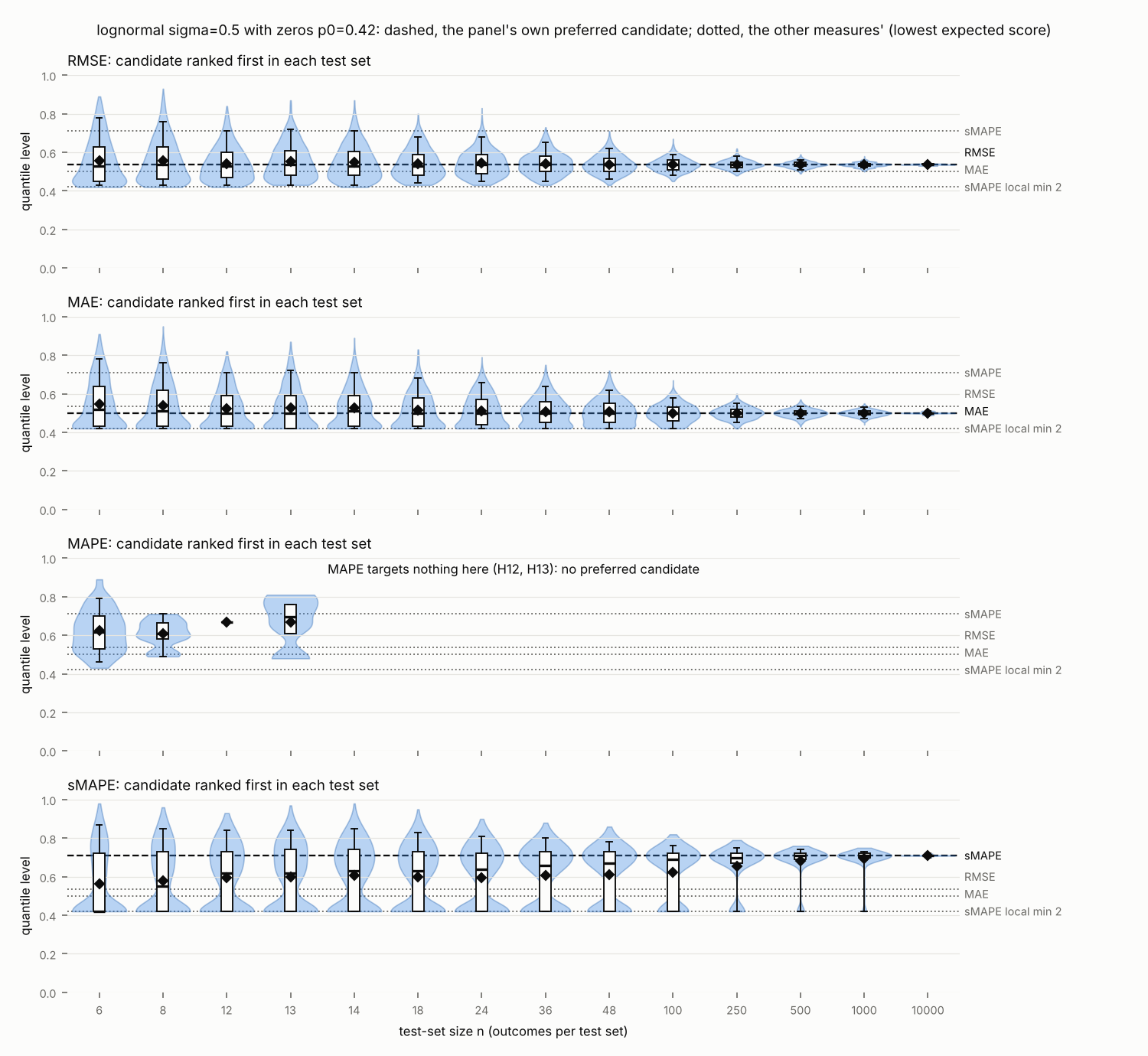
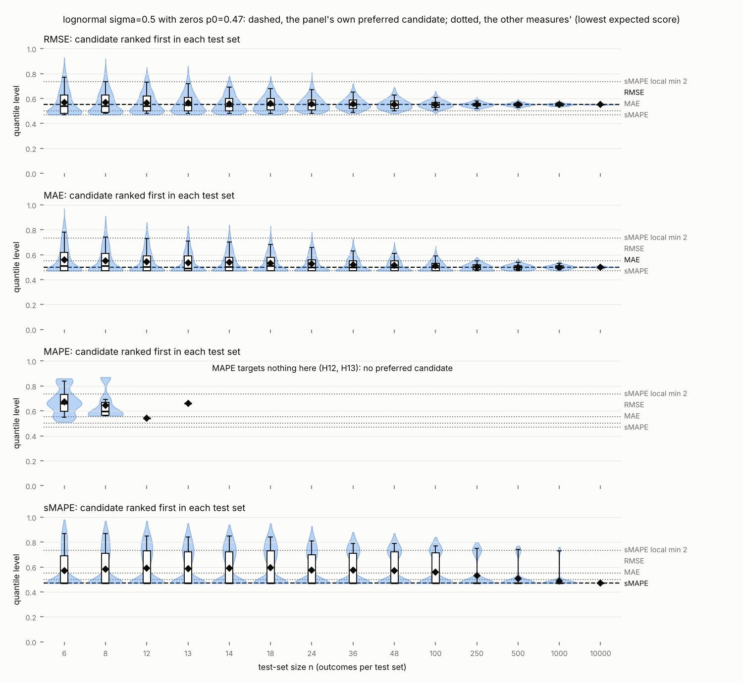
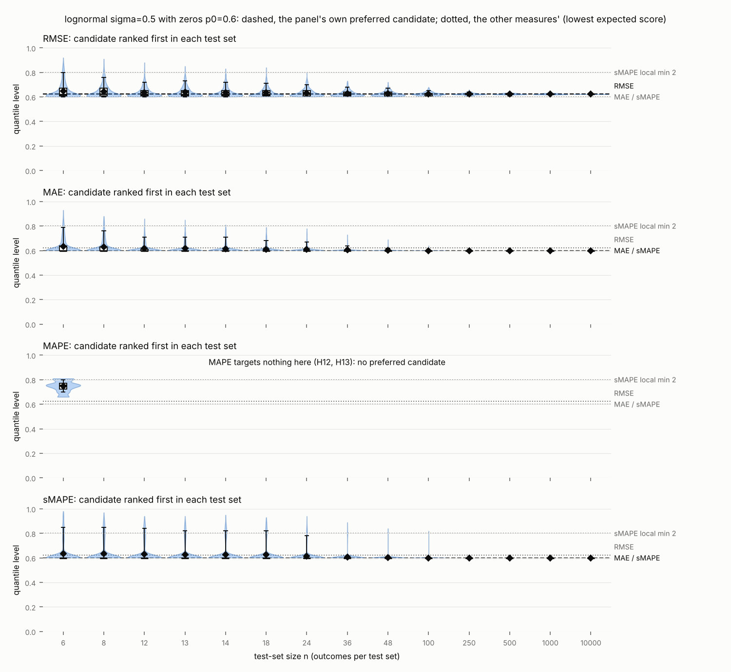
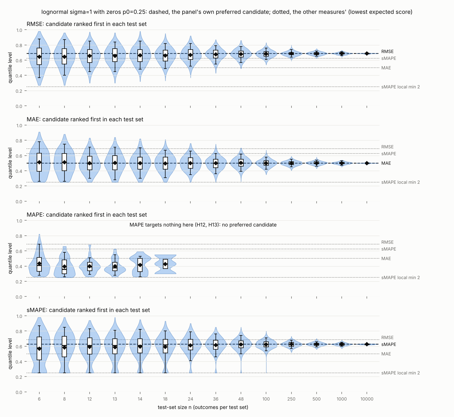
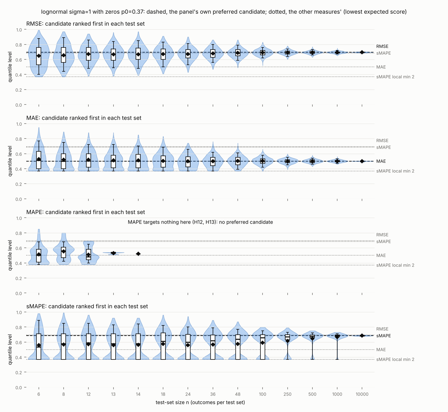
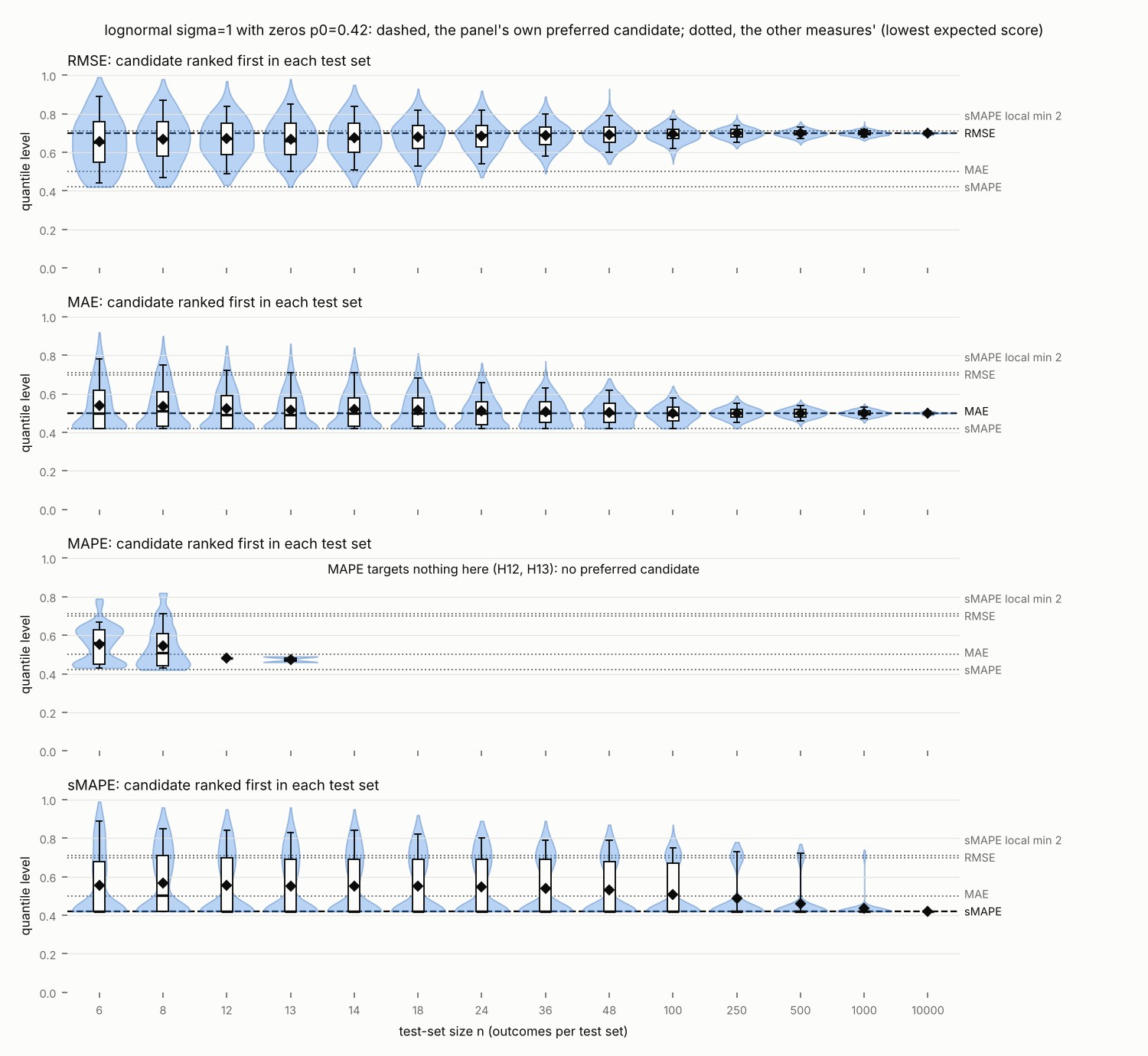
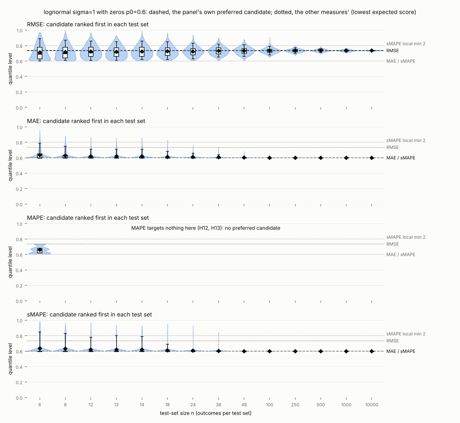
Computed from the distributions themselves, the sMAPE target on the 34 outcome distributions of plan PL1 is the median on lognormal outcomes, lies below it when is skewed right and above it when skewed left (quantile levels from 0.439 to 0.556 on the unimodal positive distributions), is two forecasts, one near each mode, on equal bimodal outcomes and the larger mode's on unequal ones, lies away from zero on the side of the mean on normal outcomes straddling zero, and switches to 0 at shares of zero outcomes from 0.343 to 0.468, all below one half. On test sets the forecast sMAPE ranks first spreads widely when they are small: on lognormal outcomes with , its quantile level runs from 0.16 to 0.82 (5th to 95th percentile over test sets) with 6 outcomes and from 0.47 to 0.53 with 1000.
Scope: data: outcome distributions given exactly (no data); conditions: 34 distributions: inverse Gaussian, log-skewed, lognormal, bimodal, normal straddling zero, zero-inflated lognormal · Data: E13 (T1.r6, T1.r14, T1.r1, T3.r20, T3.r6, T1.r29, T3.r27) · Limitations: L1 · Supports: C4 · Supports: C5 · Supports: C6 · Supports: C7 · Supports: C11 · Planned: lab plan PL1, planned 16 November 2026 · Weaknesses: the code changed after the plan
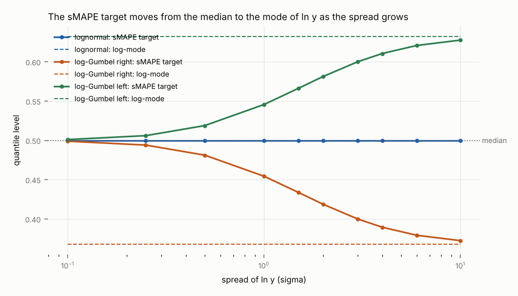
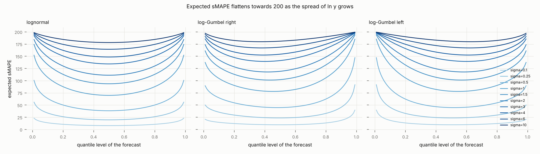
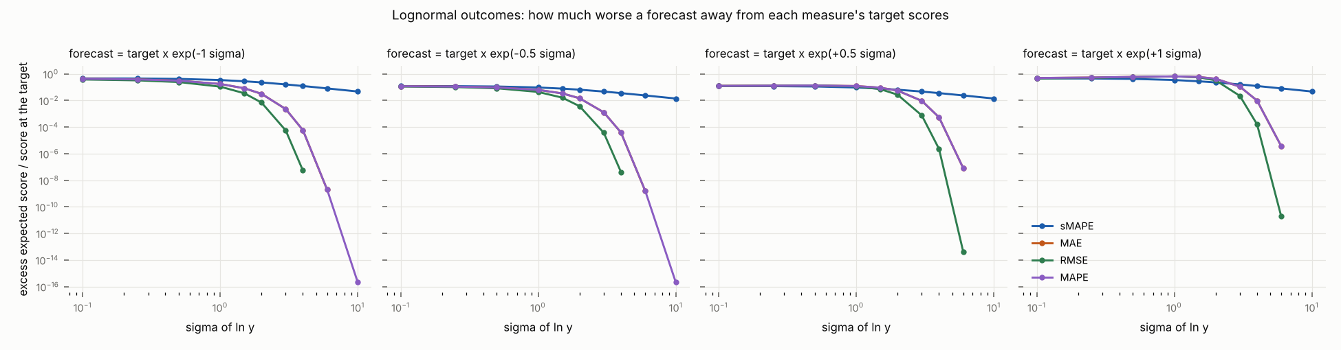
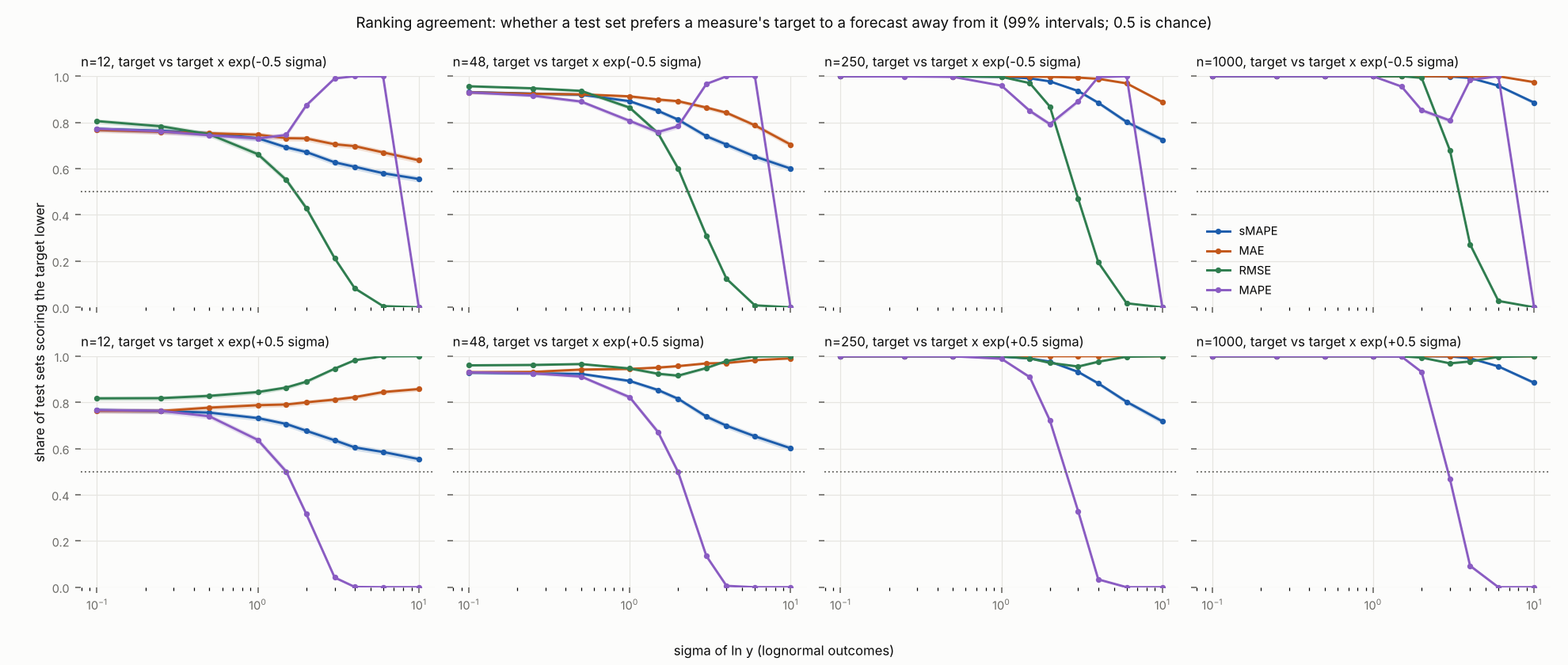
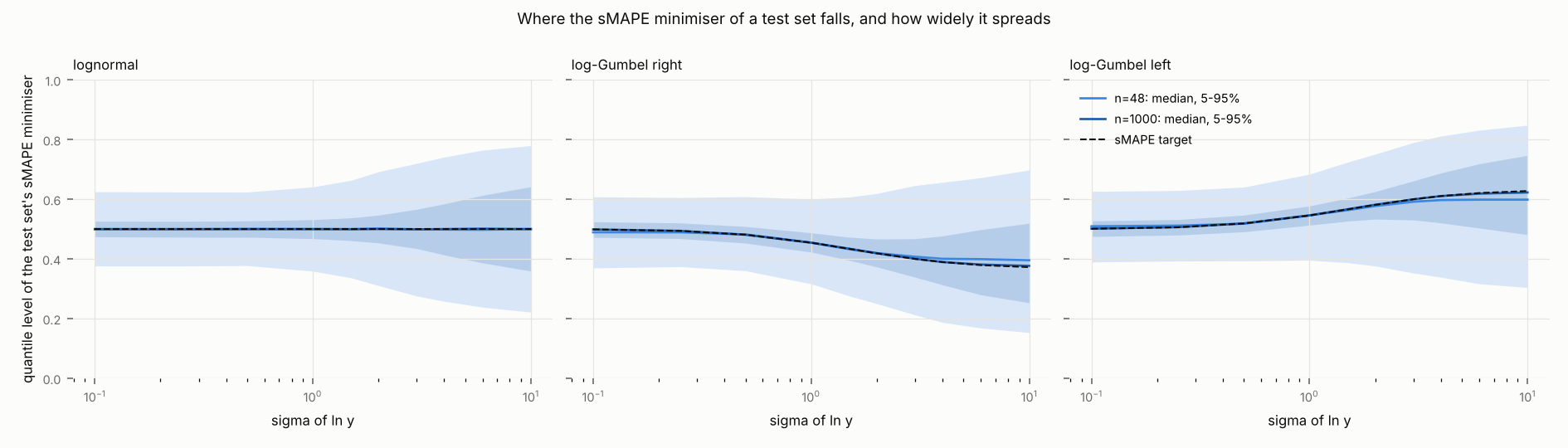
As the spread of grows from 0.1 to 10, the expected sMAPE at the sMAPE target rises towards its bound 200 (from 7.97 to 178.2 on lognormal outcomes), the target's quantile level moves from the median to that of the mode of (0.372 against the mode's 0.368 at on log-Gumbel outcomes skewed right), and the ranking agreement of sMAPE, for its target against a forecast half a away, is lower than that of MAE: at with test sets of 12 outcomes it ranks its target first in 0.61 of the test sets, MAE in 0.82.
Scope: data: outcome distributions given exactly, and test sets drawn from them; conditions: lognormal and log-Gumbel outcomes, spread of ln y from 0.1 to 10, test sets of 12 to 1000 outcomes · Data: E14 (T1.r1, T1.r28, T1.r29, T1.r2, T1.r24, T2.r5) · Supports: C10 · Planned: lab plan PL4, planned 16 November 2026
Computed from the distributions themselves, the Suilin target differs little from the sMAPE target away from zero and on counts, and differs near zero: it is within 0.3% of the sMAPE target on the six distributions with median about 100, and the same as the sMAPE target on every Poisson counts distribution studied; on lognormal actuals with median 1 and it is 0.985 instead of 1, and the share of zeros at which it switches to the forecast 0 is 0.470 instead of sMAPE's 0.394, while at median 100 the two shares are 0.3937 and 0.3940.
Scope: data: outcome distributions given exactly (no data); conditions: positive distributions at median about 100, lognormal with zeros at medians 1 and 100, Poisson counts with means 0.3 to 10 · Data: E16 (T1.r7, T2.r1, T2.r2) · Supports: C17 · Planned: lab plan PL11, planned 17 November 2026
The forecasts that sMAPE, msMAPE with , 0.5 and 1, and the Suilin loss reward were computed from the distributions themselves on the 14 intermittent demand settings. (a) On each of the 10 count distributions, the msMAPE target with and the Suilin target equal the sMAPE target. With the msMAPE target is 1 instead of 0 on Poisson counts with mean 0.7 and on negative binomial counts with mean 2, and 1 instead of 2 on Poisson counts with mean 1.5. With it is also 1 instead of 0 on Poisson counts with mean 0.5 and on negative binomial counts with mean 1. (b) For lognormal demand sizes with zeros, the share of zeros at which the target switches to the forecast 0 is 0.394 for sMAPE, 0.419 for msMAPE with , 0.470 for the Suilin loss, 0.519 for msMAPE with and 0.565 with . (c) In test sets of 12, 52 and 365 actuals, the forecast with the lowest score is 0 no more often under msMAPE than under sMAPE, and no more often under a larger . With 52 actuals from Poisson counts with mean 0.7, it is 0 in 0.6575 of the test sets under sMAPE, 0.523 with , 0.1525 with and 0.0265 with .
Scope: data: outcome distributions given exactly, and test sets drawn from them; conditions: 14 settings: 10 count distributions (Poisson with means 0.1 to 3, negative binomial with size 0.5 and means 0.5 to 2) and lognormal demand sizes (median 1, sigma 1) with shares of zeros 0.2 to 0.8, msMAPE with nu = 0.1, 0.5 and 1, test sets of 12, 52 and 365 independent actuals, 2000 test sets per setting and size · Data: E34 (T1.r1, T1.r2, T1.r3, T1.r4, T1.r5, T1.r6, T1.r7, T1.r8, T1.r9, T1.r10, T2.r1, T4, T4.r11) · Supports: C20 · Planned: lab plan PL14, planned 18 November 2026
Evidence
Numerical checks of the formulas of the formal claims (formula checks), lab run RN8 under the formal plan that decided them; every check is within the plan's tolerances. They check the formulas on concrete numbers; the proofs are the evidence for the claims. The rows are labelled by the hypotheses of the record's first plan, whose wording kept the factor 200: H1 checks C1; H2 and H10 check C2; H5 checks C5; H7 checks C6; H8 checks C7; H12 checks C8; H13 checks C9; H14 checks C10. H3 and H9 checked C3, and H4 and H6 checked C4, as version 2 worded them; C3, C4 and C12 as now worded are checked in E31. The two results E1.R1 and E1.R2 compare a simulated variance with the large-sample variance that C19 now proves.
Setup: studied sMAPE term, expected sMAPE, log error, weight, sMAPE target · procedure formula checks
- R1 simulated n Var(ln sMAPE minimiser) / large-sample value, lognormal sigma=1 = 0.9944 99% confidence interval 0.9354 to 1.0598 (hypothesis: H11, test-set size: 1000, test sets: 4000)
- R2 simulated n Var(ln sMAPE minimiser) / large-sample value, lognormal sigma=1 = 1.022 99% confidence interval 0.9396 to 1.0982 (hypothesis: H11, test-set size: 10000, test sets: 2000)
- R3 maximum absolute difference from the ratio form = 0.0000 (hypothesis: H1)
- R4 maximum absolute difference between the ratio and its reciprocal = 0.0000 (hypothesis: H2)
- R5 maximum absolute difference from 200 tanh(|z|/2) = 0.0000 (hypothesis: H3)
- R6 violations of monotonicity, concavity or the bound 200 on 0 <= |z| <= 12 = 0 (hypothesis: H3)
- R7 violations of 0 <= 100|z| - s <= 25|z|^3/3 = 0 (hypothesis: H9)
- R8 maximum of |s - 100|z| + 25|z|^3/3| / |z|^5 for 0.05 < |z| < 0.5 = 0.8331 (hypothesis: H9)
- R9 violations of s(y, y+e) < s(y, y-e) = 0 (hypothesis: H10)
- R10 maximum absolute difference between s(y, ky) and s(y, y/k) = 0.0000 (hypothesis: H10)
- R11 maximum relative difference between the formula for S' and a numerical derivative = 0.0000 (hypothesis: H4)
- R12 maximum distance in ln f between the minimiser and the median = 0.0000 (hypothesis: H5)
- R13 number of local minima, lognormal sigma=1 and log-Laplace b=1 = 1 (hypothesis: H5)
- R14 maximum balance residual at the minimiser (pull below minus pull above) = 0.0000 (hypothesis: H6)
- R15 settings with one local minimum where the sign of D misplaces the target = 0 (hypothesis: H6)
- R16 maximum distance between the one-step and the exact quantile level = 0.0025 (hypothesis: H6)
- R17 2 g(m) - E[sech^2(Z/2) tanh(|Z|/2)] for the equal-mode bimodal setting (negative: median a local maximum) = -0.3475 (hypothesis: H7)
- R18 number of local minima of the equal-mode bimodal setting = 2 (hypothesis: H7)
- R19 difference between the two minimal expected sMAPEs, equal-mode bimodal setting = 0.0000 (hypothesis: H7)
- R20 maximum distance between the formula and the bisected threshold = 0.0000 (hypothesis: H8)
- R21 opposite-sign or one-zero pairs not scoring 200 = 0 (hypothesis: H8)
- R22 relative distance between the 1/y-weighted median and the minimiser of expected MAPE = 0.0001 (hypothesis: H12)
- R23 difference of expected squared errors minus (f1-f2)(f1+f2-2E[y]) = 0 (hypothesis: H12)
- R24 sMAPE terms outside [0, 200] = 0 (hypothesis: H13)
- R25 expected sMAPE at f = 1e-6 and f = 1e10 (both near 200) = 200 (hypothesis: H13)
- R26 the proof's bound on the error times sigma^3, 600 zeta(3) max|g''|, log-Gumbel = 309.9 (hypothesis: H14)
- R27 limit of sigma^3 times the relative efficiency for normal log-outcomes, from the proof = 7.226 (hypothesis: H14)
| Row | setting | zero threshold |
|---|---|---|
| r1 | lognormal sigma=0.3 | 0.4687 |
| r2 | lognormal sigma=0.5 | 0.4469 |
| r3 | lognormal sigma=1 | 0.394 |
| r4 | lognormal sigma=2 | 0.3075 |
| Row | sigma | maximum |S - (200 - 800 ln2 h)| times sigma^3, log-Gumbel right | sigma^3 times the asymptotic relative efficiency, lognormal |
|---|---|---|---|
| r1 | 5.0 | 264.5 | 5.613 |
| r2 | 10.0 | 292.3 | 6.743 |
| r3 | 20.0 | 300.1 | 7.099 |
| r4 | 40.0 | 302.1 | 7.193 |
Numerical checks of the formulas of C11 (formula checks), lab run RN6 under the formal plan that decided C11; every check is within the plan's tolerances. They check the formulas on concrete numbers; the proof is the evidence for the claim.
Setup: studied sMAPE target · procedure formula checks
| Row | mean | sign of the global minimiser of expected sMAPE | distance of the global minimiser from 0 | lowest expected sMAPE term | local minima of expected sMAPE | smallest distance of any local minimiser from 0 |
|---|---|---|---|---|---|---|
| r1 | -0.5 | -1 | 0.9838 | 0.5227 | 2 | 0.5849 |
| r2 | -0.2 | -1 | 0.8371 | 0.609 | 2 | 0.679 |
| r3 | -0.05 | -1 | 0.773 | 0.6525 | 2 | 0.7335 |
| r4 | -0.01 | -1 | 0.7569 | 0.664 | 2 | 0.7491 |
| r5 | 0.01 | 1 | 0.7569 | 0.664 | 2 | 0.7491 |
| r6 | 0.05 | 1 | 0.773 | 0.6525 | 2 | 0.7336 |
| r7 | 0.2 | 1 | 0.8371 | 0.609 | 2 | 0.679 |
| r8 | 0.5 | 1 | 0.9838 | 0.5227 | 2 | 0.5849 |
| Row | mean | forecast | expected sMAPE term at a forecast near 0 |
|---|---|---|---|
| r1 | -0.5 | -0.001 | 0.9948 |
| r2 | -0.5 | 0.001 | 0.9957 |
| r3 | -0.2 | -0.001 | 0.9946 |
| r4 | -0.2 | 0.001 | 0.995 |
| r5 | -0.05 | -0.001 | 0.9947 |
| r6 | -0.05 | 0.001 | 0.9948 |
| r7 | -0.01 | -0.001 | 0.9947 |
| r8 | -0.01 | 0.001 | 0.9948 |
| r9 | 0.01 | -0.001 | 0.9948 |
| r10 | 0.01 | 0.001 | 0.9947 |
| r11 | 0.05 | -0.001 | 0.9948 |
| r12 | 0.05 | 0.001 | 0.9947 |
| r13 | 0.2 | -0.001 | 0.995 |
| r14 | 0.2 | 0.001 | 0.9946 |
| r15 | 0.5 | -0.001 | 0.9957 |
| r16 | 0.5 | 0.001 | 0.9948 |
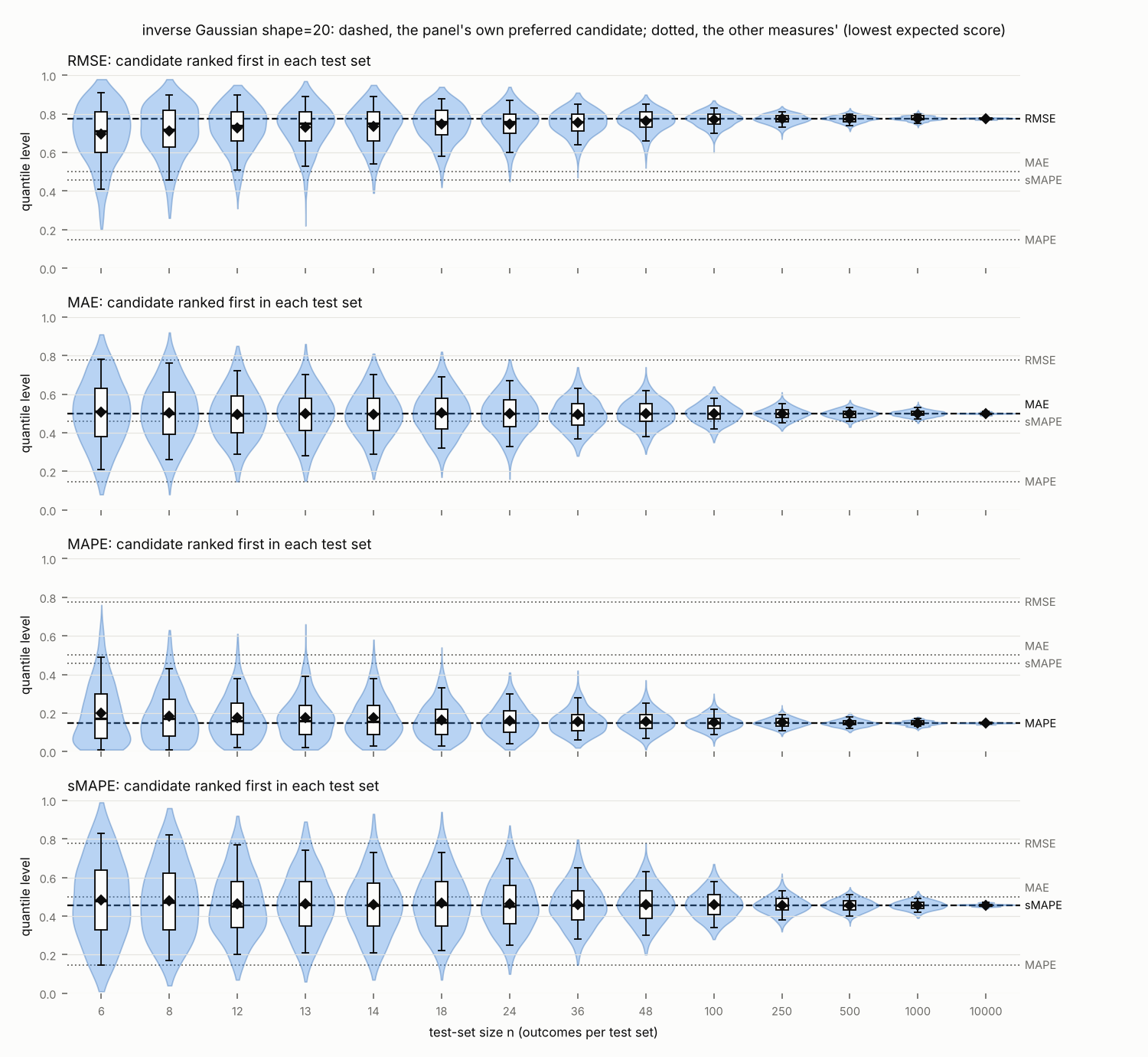
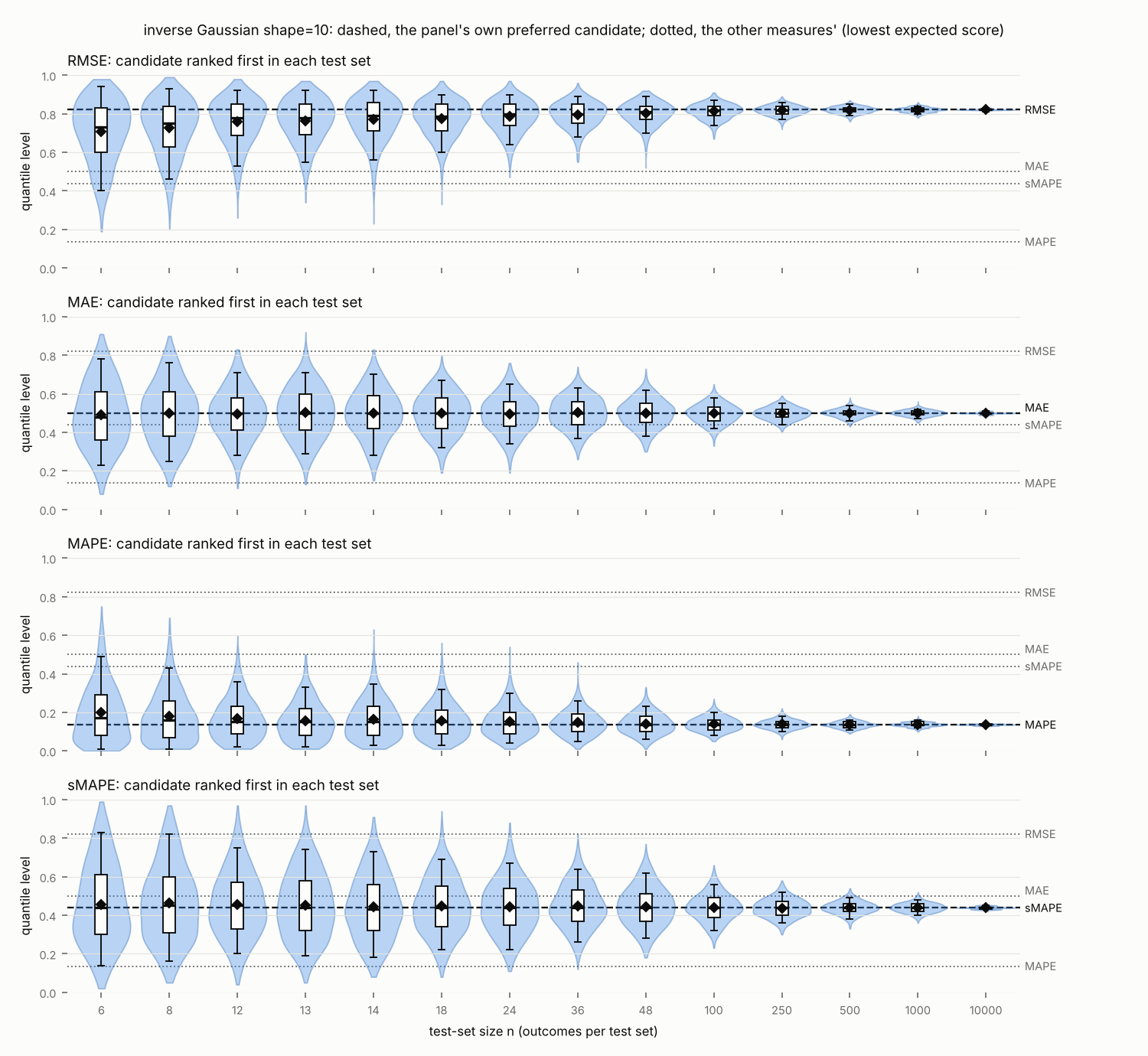
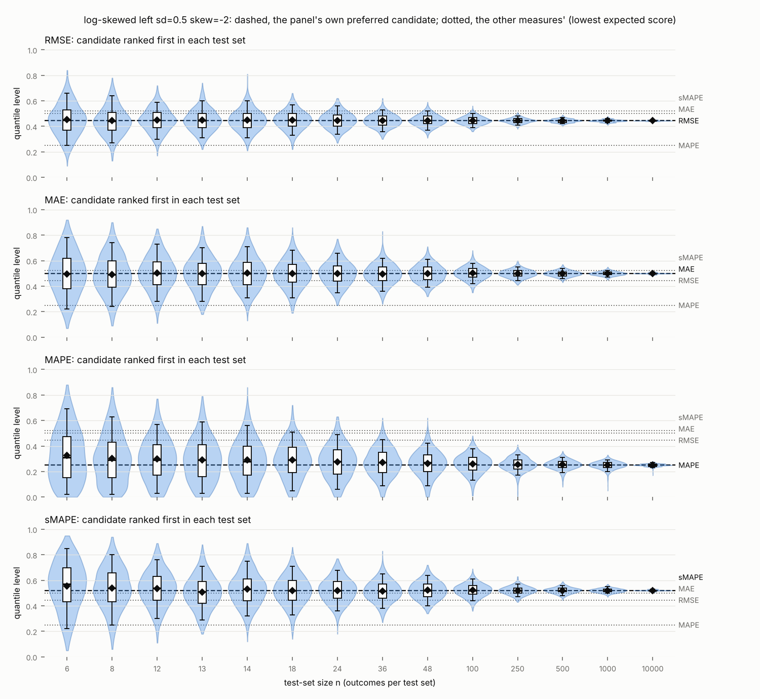
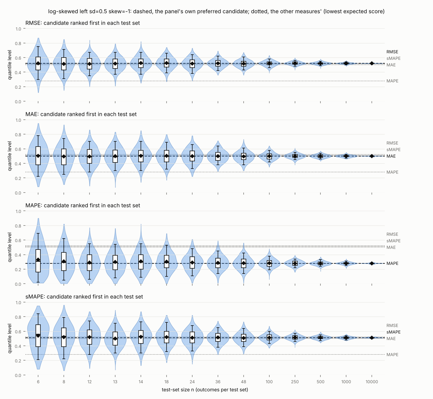
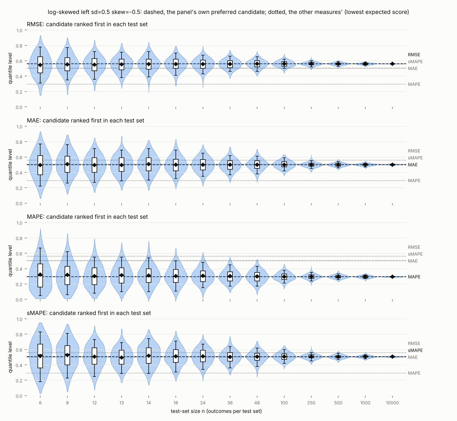
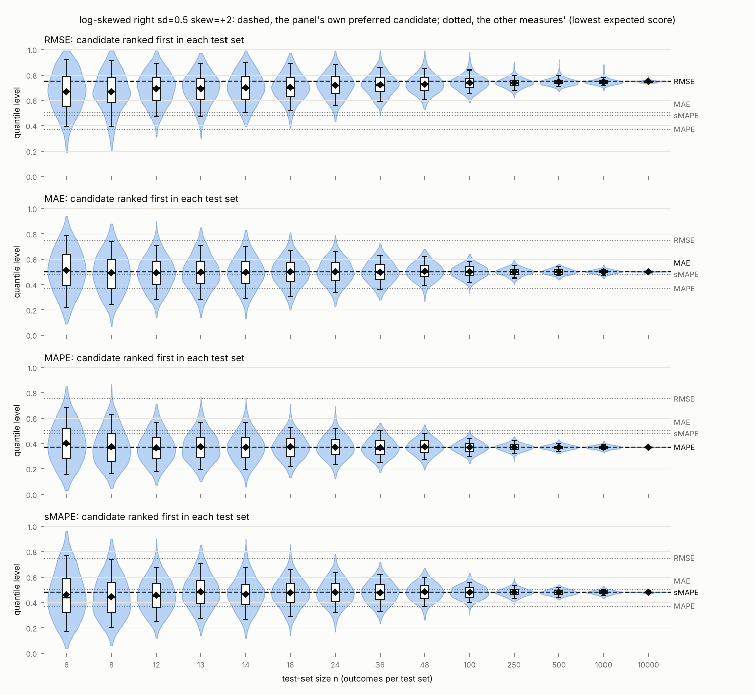
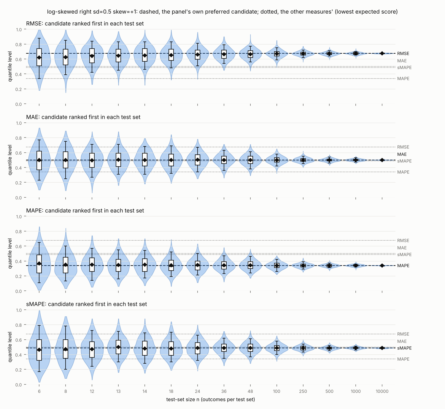
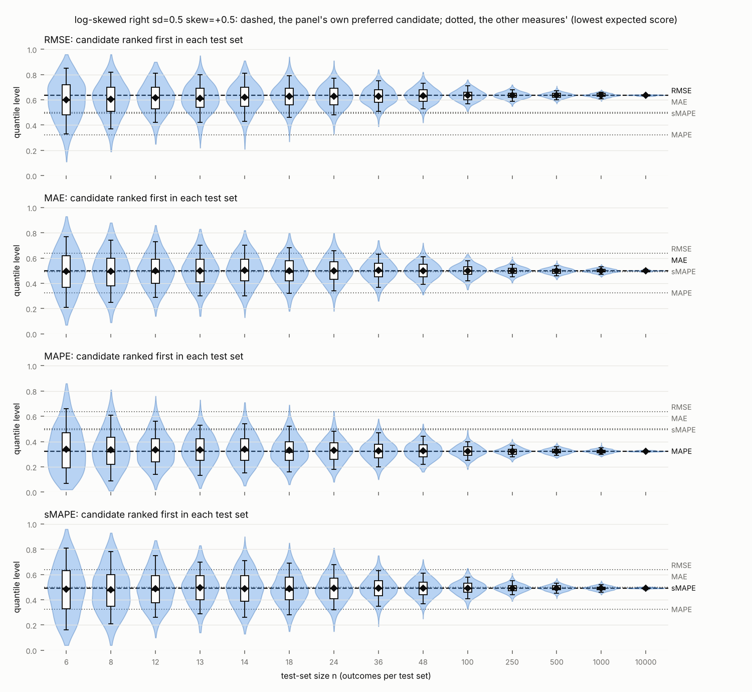
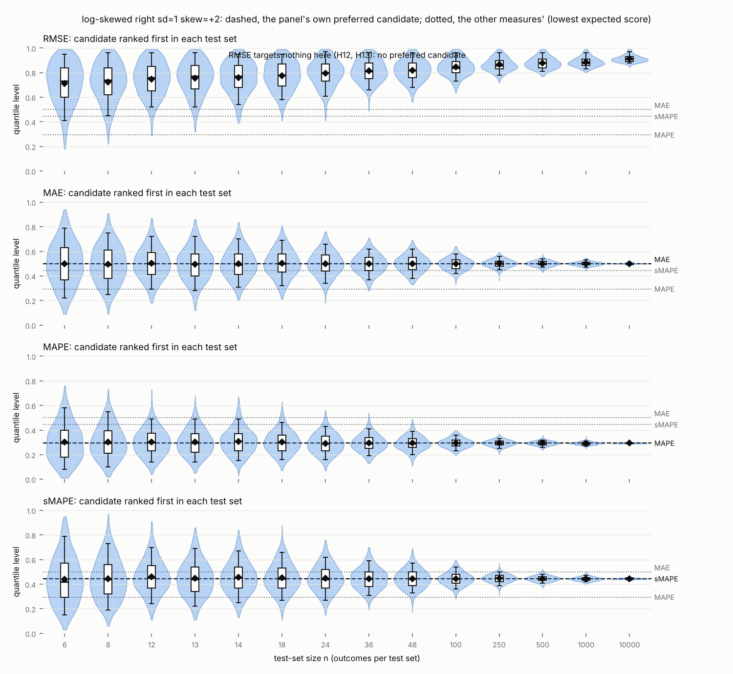
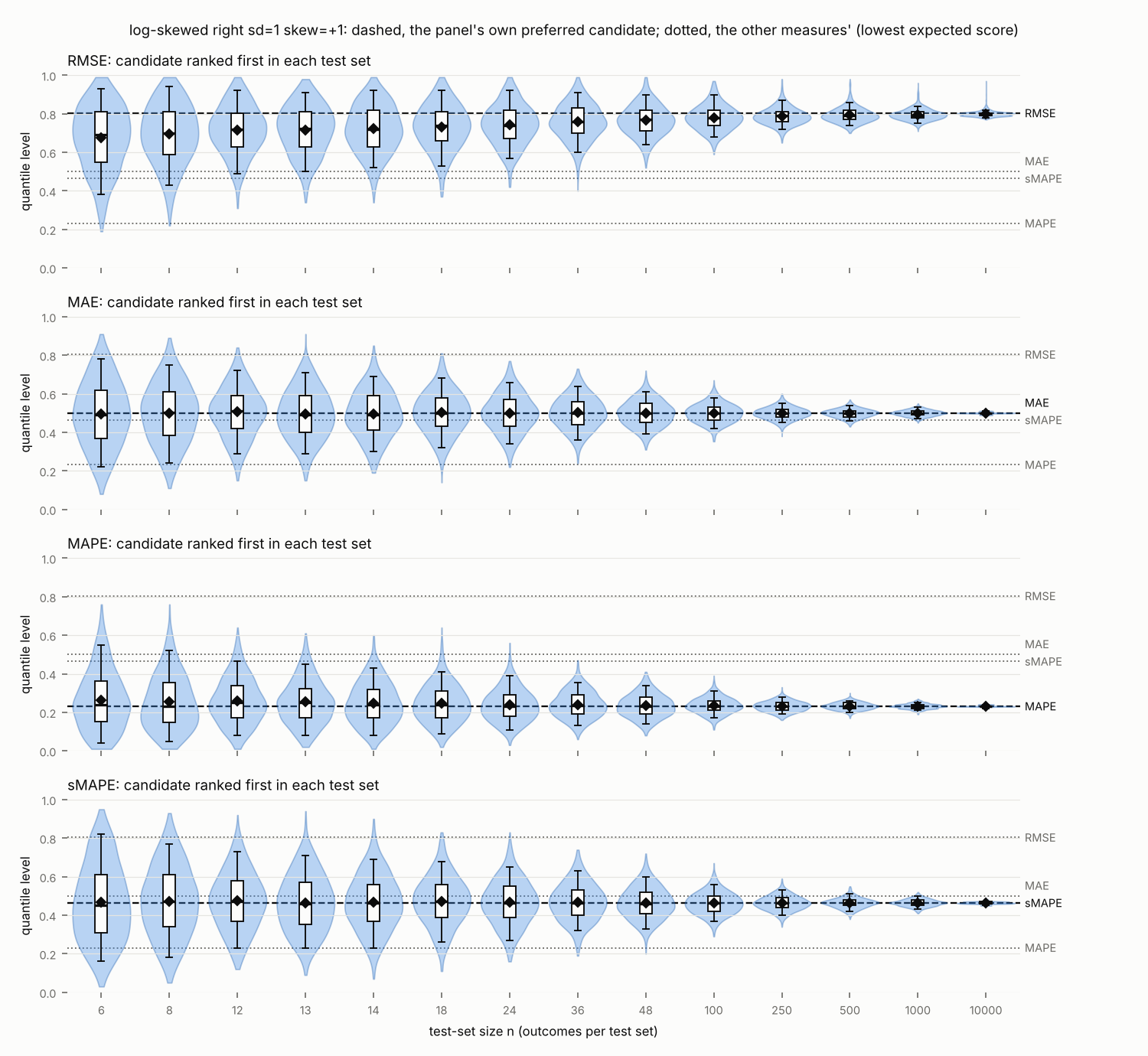
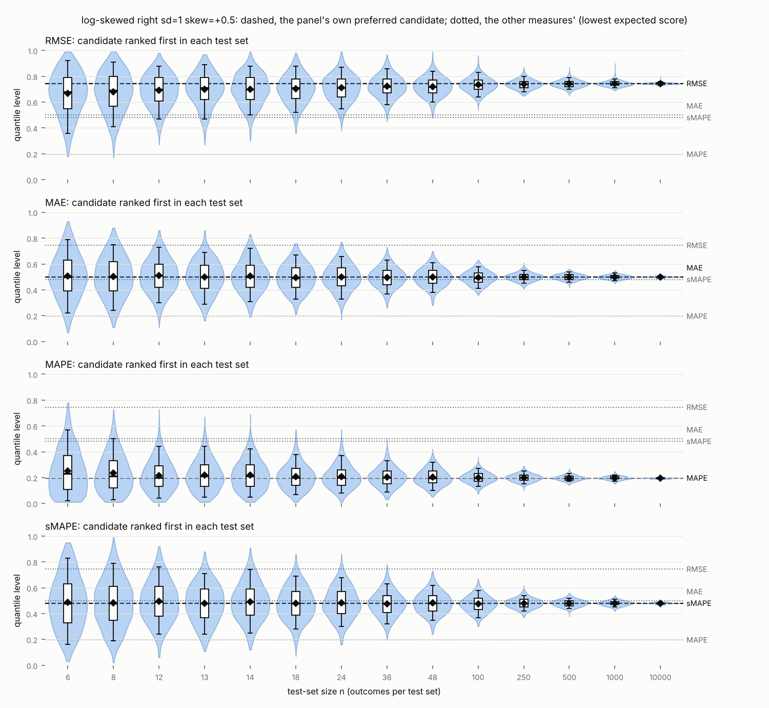
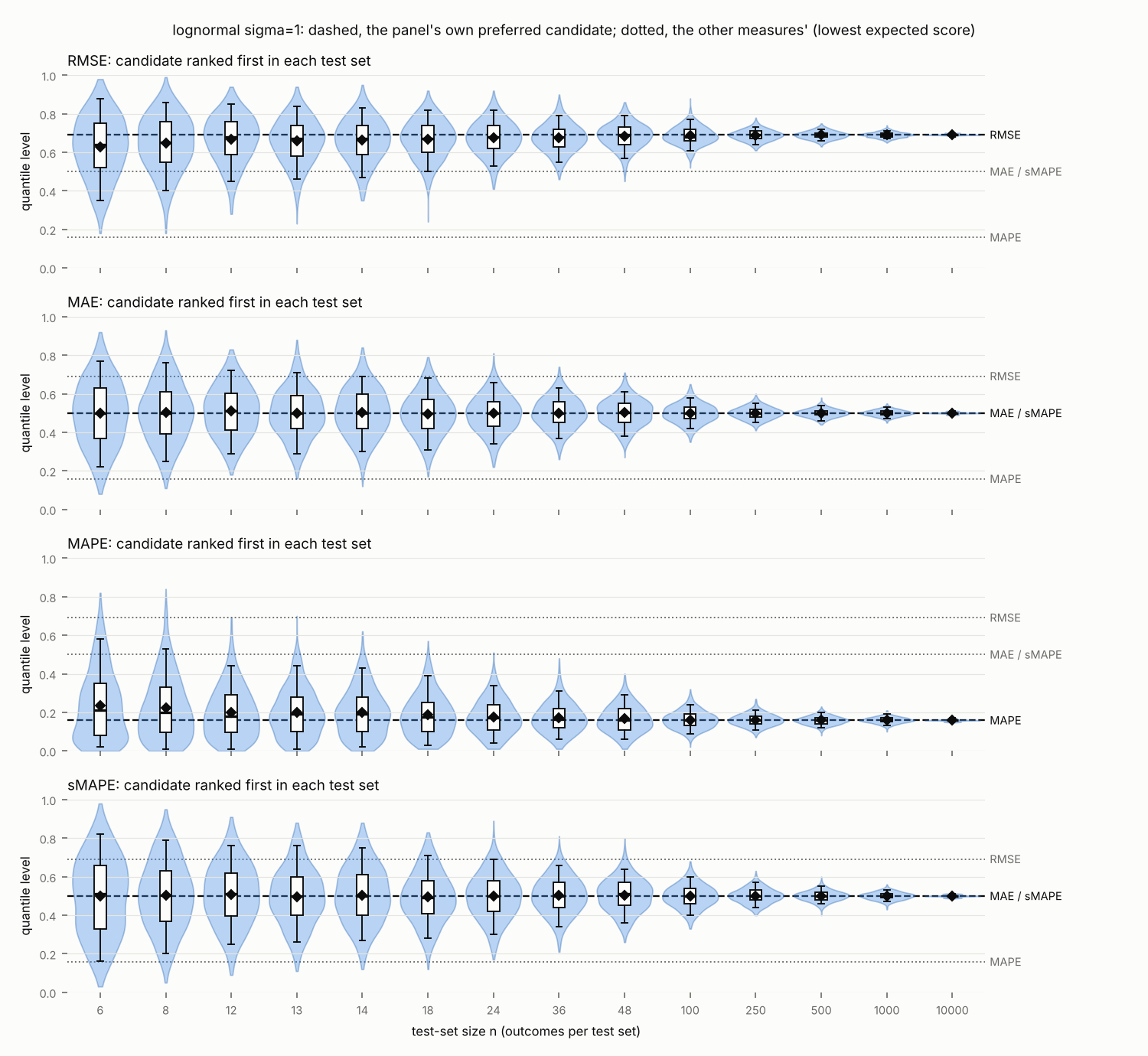
Lab runs RN1 under plan PL1. Design: Selection design (D16) on 33 outcome distributions: inverse Gaussian (6), log-skewed (12) and lognormal (2), bimodal (3), straddling zero (3), zero-inflated lognormal (8). For each: the derived values (D15) of every local minimum of expected sMAPE with its quantile level and expected score; the one-step quantile level of H6 and the pull difference D at the median; the zero threshold of H8; the quantile level of the log-mode; which moments are finite (H12); the MAPE target (H12); each measure's preferred candidate (D14), ranked by finite differences where expected scores are infinite. Candidates: quantiles at levels 0.01 to 0.99, the mean (when finite), 0, the log-mode, the MAPE minimiser (when it exists and is not 0) and every local minimiser of expected sMAPE, merged when within 1e-4 (relative). Test sets of n = 6, 8, 12, 13, 14, 18, 24, 36, 48, 100, 250, 500, 1000 and 10000 outcomes, 1000 test sets per size, seed 3 with the setting's index and n. Measures RMSE, MAE, MAPE, sMAPE on every setting. python3 claimset-code/smape-target/targets.py --seed 3 --reps 1000 (numpy 2.5.3, matplotlib 3.11.2). Analysis: Per distribution: the derived values listed in the design. Per distribution, measure and n, over test sets, of the candidate ranked first: its quantile level's mean with a 99% confidence interval and 5th, 25th, 50th, 75th and 95th percentiles; the share choosing each candidate; the share choosing the preferred candidate with its 99% Wilson interval; the number of test sets in which every candidate scores infinite. Figures: one per distribution, a panel per measure, violins of the chosen quantile levels over n with boxplots and the mean, lines at every measure's preferred candidate and at further local minima of expected sMAPE, and a note in the panel of a measure that targets nothing. These are compared with what H4 to H8, H12 and H13 predict; no test is made and no threshold is set.
Setup: studied RMSE, MAE, MAPE, sMAPE · cases inverse Gaussian outcomes, log-skewed outcomes, bimodal outcomes, outcomes straddling zero, zero-inflated outcomes · procedure selection design, derived value · lens candidate forecast, preferred candidate, sMAPE target, expected sMAPE, weight, quantile profile
| Row | setting | derived local minimum of expected sMAPE (rank: 1) | quantile level of a derived local minimum of expected sMAPE (rank: 1) | expected sMAPE at a derived local minimum (rank: 1) | one-step quantile level of the sMAPE target | pull from above minus pull from below at the median | zero threshold of sMAPE | quantile level of the log-mode | median of the outcome distribution | mean of the outcome distribution |
|---|---|---|---|---|---|---|---|---|---|---|
| r1 | inverse Gaussian shape=1000 | 95.27 | 0.4999 | 24.36 | 0.4999 | -0.0001 | 0.4676 | 0.498 | 95.27 | 100 |
| r2 | inverse Gaussian shape=200 | 80.14 | 0.4978 | 48.68 | 0.4978 | -0.0019 | 0.4307 | 0.4822 | 80.43 | 100 |
| r3 | inverse Gaussian shape=100 | 66.53 | 0.4929 | 61.97 | 0.4929 | -0.0052 | 0.4083 | 0.4597 | 67.58 | 100 |
| r4 | inverse Gaussian shape=50 | 48.86 | 0.482 | 75.05 | 0.482 | -0.0114 | 0.3845 | 0.4233 | 51.42 | 100 |
| r5 | inverse Gaussian shape=20 | 25.9 | 0.4578 | 88.96 | 0.457 | -0.0224 | 0.357 | 0.3726 | 30.11 | 100 |
| r6 | inverse Gaussian shape=10 | 14.02 | 0.4387 | 95.75 | 0.4362 | -0.03 | 0.3426 | 0.3471 | 17.85 | 100 |
| r7 | log-skewed left sd=0.5 skew=-2 | 119 | 0.5211 | 32.31 | 0.5211 | 0.0197 | 0.4561 | 1 | 116.6 | 109.9 |
| r8 | log-skewed left sd=0.5 skew=-1 | 110.2 | 0.513 | 36.74 | 0.513 | 0.0117 | 0.4494 | 0.6472 | 108.5 | 111.3 |
| r9 | log-skewed left sd=0.5 skew=-0.5 | 105.1 | 0.5068 | 37.96 | 0.5068 | 0.0061 | 0.4476 | 0.5681 | 104.2 | 112.2 |
| r10 | log-skewed right sd=0.5 skew=+2 | 84.02 | 0.4789 | 32.31 | 0.4789 | -0.0197 | 0.4561 | 0 | 85.78 | 121.3 |
| r11 | log-skewed right sd=0.5 skew=+1 | 90.72 | 0.487 | 36.74 | 0.487 | -0.0117 | 0.4494 | 0.3528 | 92.13 | 116.3 |
| r12 | log-skewed right sd=0.5 skew=+0.5 | 95.13 | 0.4932 | 37.96 | 0.4932 | -0.0061 | 0.4476 | 0.4319 | 95.93 | 114.6 |
| r13 | lognormal sigma=0.5 | 100 | 0.5 | 38.38 | 0.5 | 0.0000 | 0.4469 | 0.5 | 100 | 113.3 |
| r14 | log-skewed left sd=1 skew=-2 | 151.2 | 0.5562 | 57.04 | 0.5572 | 0.0456 | 0.4168 | 1 | 135.9 | 135.9 |
| r15 | log-skewed left sd=1 skew=-1 | 128.3 | 0.5362 | 66.42 | 0.5365 | 0.0261 | 0.4004 | 0.6472 | 117.8 | 146 |
| r16 | log-skewed left sd=1 skew=-0.5 | 113.9 | 0.5191 | 69.05 | 0.5192 | 0.0133 | 0.3957 | 0.5681 | 108.7 | 153.7 |
| r17 | log-skewed right sd=1 skew=+2 | 66.14 | 0.4438 | 57.04 | 0.4428 | -0.0456 | 0.4168 | 0 | 73.58 | |
| r18 | log-skewed right sd=1 skew=+1 | 77.96 | 0.4638 | 66.42 | 0.4635 | -0.0261 | 0.4004 | 0.3528 | 84.88 | 216.5 |
| r19 | log-skewed right sd=1 skew=+0.5 | 87.79 | 0.4809 | 69.05 | 0.4808 | -0.0133 | 0.3957 | 0.4319 | 92.03 | 182.7 |
| r20 | lognormal sigma=1 | 100 | 0.5 | 69.94 | 0.5 | 0.0000 | 0.394 | 0.5 | 100 | 164.9 |
| r21 | bimodal equal modes | 43.49 | 0.3742 | 83.84 | 0.5 | 0.0000 | 0.3674 | 0.25 | 100 | 159.2 |
| r22 | bimodal left mode higher | 39.84 | 0.4063 | 65.21 | 0.4042 | -0.0839 | 0.4026 | 0.325 | 44.22 | 122.8 |
| r23 | bimodal right mode higher | 251 | 0.5937 | 65.21 | 0.5958 | 0.0839 | 0.4026 | 0.675 | 226.1 | 195.6 |
| r24 | normal straddling zero mean=0 | -0.753 | 0.2257 | 133.4 | 0.0000 | 0 | ||||
| r25 | normal straddling zero mean=0.5 | 0.9838 | 0.6858 | 104.5 | 0.5 | 0.5 | ||||
| r26 | normal straddling zero mean=1 | 1.287 | 0.6128 | 78.51 | 1 | 1 | ||||
| r27 | lognormal sigma=0.5 with zeros p0=0.25 | 100 | 0.625 | 78.78 | 0.5 | 0.0000 | 0.4469 | 0.625 | 80.62 | 84.99 |
| r28 | lognormal sigma=0.5 with zeros p0=0.42 | 100 | 0.71 | 106.3 | 0.5 | 0.0000 | 0.4469 | 0.71 | 57.99 | 65.72 |
| r29 | lognormal sigma=0.5 with zeros p0=0.47 | 0 | 0.47 | 106 | 0.5 | 0.0000 | 0.4469 | 0.735 | 45.3 | 60.06 |
| r30 | lognormal sigma=0.5 with zeros p0=0.6 | 0 | 0.6 | 80 | 0.5 | 0.0000 | 0.4469 | 0.8 | 0 | 45.33 |
| r31 | lognormal sigma=1 with zeros p0=0.25 | 100 | 0.625 | 102.5 | 0.5 | 0.0000 | 0.394 | 0.625 | 65 | 123.7 |
| r32 | lognormal sigma=1 with zeros p0=0.37 | 100 | 0.685 | 118.1 | 0.5 | 0.0000 | 0.394 | 0.685 | 44.08 | 103.9 |
| r33 | lognormal sigma=1 with zeros p0=0.42 | 0 | 0.42 | 116 | 0.5 | 0.0000 | 0.394 | 0.71 | 33.63 | 95.63 |
| r34 | lognormal sigma=1 with zeros p0=0.6 | 0 | 0.6 | 80 | 0.5 | 0.0000 | 0.394 | 0.8 | 0 | 65.95 |
| Row | setting | derived local minimum of expected sMAPE (rank: 2) | quantile level of a derived local minimum of expected sMAPE (rank: 2) | expected sMAPE at a derived local minimum (rank: 2) |
|---|---|---|---|---|
| r1 | bimodal equal modes | 229.9 | 0.6258 | 83.84 |
| r2 | normal straddling zero mean=0 | 0.753 | 0.7743 | 133.4 |
| r3 | normal straddling zero mean=0.5 | -0.5849 | 0.139 | 159.9 |
| r4 | normal straddling zero mean=1 | -0.4649 | 0.0715 | 179.8 |
| r5 | lognormal sigma=0.5 with zeros p0=0.25 | 0 | 0.25 | 150 |
| r6 | lognormal sigma=0.5 with zeros p0=0.42 | 0 | 0.42 | 116 |
| r7 | lognormal sigma=0.5 with zeros p0=0.47 | 100 | 0.735 | 114.3 |
| r8 | lognormal sigma=0.5 with zeros p0=0.6 | 100 | 0.8 | 135.4 |
| r9 | lognormal sigma=1 with zeros p0=0.25 | 0 | 0.25 | 150 |
| r10 | lognormal sigma=1 with zeros p0=0.37 | 0 | 0.37 | 126 |
| r11 | lognormal sigma=1 with zeros p0=0.42 | 100 | 0.71 | 124.6 |
| r12 | lognormal sigma=1 with zeros p0=0.6 | 100 | 0.8 | 148 |
| Row | setting | quantile level of the preferred candidate (measure: RMSE) | quantile level of the preferred candidate (measure: MAE) | quantile level of the preferred candidate (measure: MAPE) | quantile level of the preferred candidate (measure: sMAPE) | candidates whose expected score is infinite (measure: RMSE) | candidates whose expected score is infinite (measure: MAPE) |
|---|---|---|---|---|---|---|---|
| r1 | inverse Gaussian shape=1000 | 0.5616 | 0.4999 | 0.3786 | 0.4999 | 0 | 0 |
| r2 | inverse Gaussian shape=200 | 0.6277 | 0.5 | 0.2659 | 0.4978 | 0 | 0 |
| r3 | inverse Gaussian shape=100 | 0.6681 | 0.5 | 0.2158 | 0.4929 | 0 | 0 |
| r4 | inverse Gaussian shape=50 | 0.7138 | 0.5 | 0.1773 | 0.482 | 0 | 0 |
| r5 | inverse Gaussian shape=20 | 0.7768 | 0.5 | 0.1474 | 0.4578 | 0 | 0 |
| r6 | inverse Gaussian shape=10 | 0.8219 | 0.5 | 0.136 | 0.4387 | 0 | 0 |
| r7 | log-skewed left sd=0.5 skew=-2 | 0.4444 | 0.5 | 0.25 | 0.5211 | 0 | 0 |
| r8 | log-skewed left sd=0.5 skew=-1 | 0.5215 | 0.5 | 0.2799 | 0.513 | 0 | 0 |
| r9 | log-skewed left sd=0.5 skew=-0.5 | 0.5603 | 0.5 | 0.2941 | 0.5068 | 0 | 0 |
| r10 | log-skewed right sd=0.5 skew=+2 | 0.75 | 0.5 | 0.37 | 0.4789 | 102 | 0 |
| r11 | log-skewed right sd=0.5 skew=+1 | 0.6748 | 0.5 | 0.3388 | 0.487 | 0 | 0 |
| r12 | log-skewed right sd=0.5 skew=+0.5 | 0.6368 | 0.5 | 0.3234 | 0.4932 | 0 | 0 |
| r13 | lognormal sigma=0.5 | 0.5987 | 0.5 | 0.3085 | 0.5 | 0 | 0 |
| r14 | log-skewed left sd=1 skew=-2 | 0.5 | 0.5 | 0 | 0.5562 | 0 | 101 |
| r15 | log-skewed left sd=1 skew=-1 | 0.5928 | 0.5 | 0.0655 | 0.5362 | 0 | 0 |
| r16 | log-skewed left sd=1 skew=-0.5 | 0.6413 | 0.5 | 0.1155 | 0.5191 | 0 | 0 |
| r17 | log-skewed right sd=1 skew=+2 | 0.5 | 0.2929 | 0.4438 | 103 | 0 | |
| r18 | log-skewed right sd=1 skew=+1 | 0.8034 | 0.5 | 0.2314 | 0.4638 | 104 | 0 |
| r19 | log-skewed right sd=1 skew=+0.5 | 0.7446 | 0.5 | 0.1968 | 0.4809 | 0 | 0 |
| r20 | lognormal sigma=1 | 0.6915 | 0.5 | 0.1587 | 0.5 | 0 | 0 |
| r21 | bimodal equal modes | 0.5081 | 0.5 | 0.2341 | 0.3742 | 0 | 0 |
| r22 | bimodal left mode higher | 0.6503 | 0.5 | 0.2841 | 0.4063 | 0 | 0 |
| r23 | bimodal right mode higher | 0.4111 | 0.5 | 0.1848 | 0.5937 | 0 | 0 |
| r24 | normal straddling zero mean=0 | 0.5 | 0.5 | 0.5 | 0.7743 | 0 | 100 |
| r25 | normal straddling zero mean=0.5 | 0.5 | 0.5 | 0.3085 | 0.6858 | 0 | 101 |
| r26 | normal straddling zero mean=1 | 0.5 | 0.5 | 0.1587 | 0.6128 | 0 | 101 |
| r27 | lognormal sigma=0.5 with zeros p0=0.25 | 0.5293 | 0.5 | 0.625 | 0 | 77 | |
| r28 | lognormal sigma=0.5 with zeros p0=0.42 | 0.5364 | 0.5 | 0.71 | 0 | 59 | |
| r29 | lognormal sigma=0.5 with zeros p0=0.47 | 0.5516 | 0.5 | 0.47 | 0 | 55 | |
| r30 | lognormal sigma=0.5 with zeros p0=0.6 | 0.6227 | 0.6 | 0.6 | 0 | 41 | |
| r31 | lognormal sigma=1 with zeros p0=0.25 | 0.6881 | 0.5 | 0.625 | 0 | 77 | |
| r32 | lognormal sigma=1 with zeros p0=0.37 | 0.6945 | 0.5 | 0.685 | 0 | 65 | |
| r33 | lognormal sigma=1 with zeros p0=0.42 | 0.6997 | 0.5 | 0.42 | 0 | 59 | |
| r34 | lognormal sigma=1 with zeros p0=0.6 | 0.7354 | 0.6 | 0.6 | 0 | 41 |
| Row | setting | measure | test-set size | mean quantile level of the chosen candidates | percentile of the chosen candidates' quantile levels (percentile: 5) | percentile of the chosen candidates' quantile levels (percentile: 50) | percentile of the chosen candidates' quantile levels (percentile: 95) | share of test sets choosing the preferred candidate | test sets in which every candidate's score is infinite |
|---|---|---|---|---|---|---|---|---|---|
| r1 | lognormal sigma=1 | RMSE | 6 | 0.6287 | 0.3495 | 0.64 | 0.88 | 0.012 | |
| r2 | lognormal sigma=1 | RMSE | 100 | 0.6868 | 0.61 | 0.68 | 0.77 | 0.041 | |
| r3 | lognormal sigma=1 | RMSE | 1000 | 0.6911 | 0.67 | 0.6915 | 0.7105 | 0.14 | |
| r4 | lognormal sigma=1 | MAE | 6 | 0.4987 | 0.2264 | 0.505 | 0.7566 | 0.0222 | |
| r5 | lognormal sigma=1 | MAE | 100 | 0.4987 | 0.42 | 0.5 | 0.58 | 0.0733 | |
| r6 | lognormal sigma=1 | MAE | 1000 | 0.5002 | 0.47 | 0.5 | 0.53 | 0.256 | |
| r7 | lognormal sigma=1 | MAPE | 6 | 0.237 | 0.0195 | 0.21 | 0.5805 | 0.006 | |
| r8 | lognormal sigma=1 | MAPE | 100 | 0.1614 | 0.09 | 0.1587 | 0.24 | 0.041 | |
| r9 | lognormal sigma=1 | MAPE | 1000 | 0.1594 | 0.13 | 0.16 | 0.19 | 0.123 | |
| r10 | lognormal sigma=1 | sMAPE | 6 | 0.4988 | 0.16 | 0.51 | 0.82 | 0.007 | |
| r11 | lognormal sigma=1 | sMAPE | 100 | 0.4991 | 0.4 | 0.5 | 0.6 | 0.063 | |
| r12 | lognormal sigma=1 | sMAPE | 1000 | 0.5003 | 0.47 | 0.5 | 0.53 | 0.201 | |
| r13 | inverse Gaussian shape=10 | RMSE | 6 | 0.7076 | 0.4 | 0.73 | 0.94 | 0.014 | |
| r14 | inverse Gaussian shape=10 | RMSE | 100 | 0.8129 | 0.74 | 0.82 | 0.87 | 0.053 | |
| r15 | inverse Gaussian shape=10 | RMSE | 1000 | 0.8203 | 0.8 | 0.8219 | 0.84 | 0.175 | |
| r16 | inverse Gaussian shape=10 | MAE | 6 | 0.49 | 0.2355 | 0.48 | 0.7677 | 0.0192 | |
| r17 | inverse Gaussian shape=10 | MAE | 100 | 0.4979 | 0.415 | 0.5 | 0.58 | 0.09 | |
| r18 | inverse Gaussian shape=10 | MAE | 1000 | 0.5 | 0.47 | 0.5 | 0.52 | 0.25 | |
| r19 | inverse Gaussian shape=10 | MAPE | 6 | 0.1991 | 0.01 | 0.17 | 0.49 | 0.008 | |
| r20 | inverse Gaussian shape=10 | MAPE | 100 | 0.1397 | 0.08 | 0.136 | 0.2 | 0.049 | |
| r21 | inverse Gaussian shape=10 | MAPE | 1000 | 0.1369 | 0.12 | 0.136 | 0.16 | 0.157 | |
| r22 | inverse Gaussian shape=10 | sMAPE | 6 | 0.4576 | 0.1398 | 0.4387 | 0.8305 | 0.008 | |
| r23 | inverse Gaussian shape=10 | sMAPE | 100 | 0.4392 | 0.32 | 0.4387 | 0.56 | 0.025 | |
| r24 | inverse Gaussian shape=10 | sMAPE | 1000 | 0.439 | 0.4 | 0.4387 | 0.48 | 0.084 | |
| r25 | bimodal equal modes | RMSE | 6 | 0.5355 | 0.49 | 0.5081 | 0.69 | 0.223 | |
| r26 | bimodal equal modes | RMSE | 100 | 0.5121 | 0.5081 | 0.5081 | 0.53 | 0.53 | |
| r27 | bimodal equal modes | RMSE | 1000 | 0.5088 | 0.5081 | 0.5081 | 0.51 | 0.65 | |
| r28 | bimodal equal modes | MAE | 6 | 0.4963 | 0.226 | 0.4967 | 0.76 | 0.017 | |
| r29 | bimodal equal modes | MAE | 100 | 0.5012 | 0.42 | 0.506 | 0.5852 | 0.0431 | |
| r30 | bimodal equal modes | MAE | 1000 | 0.4994 | 0.47 | 0.5 | 0.53 | 0.06 | |
| r31 | bimodal equal modes | MAPE | 6 | 0.255 | 0.04 | 0.25 | 0.47 | 0.011 | |
| r32 | bimodal equal modes | MAPE | 100 | 0.2342 | 0.18 | 0.2341 | 0.29 | 0.056 | |
| r33 | bimodal equal modes | MAPE | 1000 | 0.2344 | 0.21 | 0.2341 | 0.25 | 0.164 | |
| r34 | bimodal equal modes | sMAPE | 6 | 0.4952 | 0.14 | 0.47 | 0.84 | 0.011 | |
| r35 | bimodal equal modes | sMAPE | 100 | 0.5065 | 0.31 | 0.585 | 0.7 | 0.024 | |
| r36 | bimodal equal modes | sMAPE | 1000 | 0.4998 | 0.35 | 0.6 | 0.65 | 0.077 | |
| r37 | lognormal sigma=1 with zeros p0=0.42 | RMSE | 6 | 0.6545 | 0.44 | 0.65 | 0.89 | 0.013 | |
| r38 | lognormal sigma=1 with zeros p0=0.42 | RMSE | 100 | 0.6942 | 0.62 | 0.69 | 0.77 | 0.052 | |
| r39 | lognormal sigma=1 with zeros p0=0.42 | RMSE | 1000 | 0.699 | 0.68 | 0.6997 | 0.72 | 0.124 | |
| r40 | lognormal sigma=1 with zeros p0=0.42 | MAE | 6 | 0.5375 | 0.42 | 0.51 | 0.7502 | 0.0227 | |
| r41 | lognormal sigma=1 with zeros p0=0.42 | MAE | 100 | 0.4988 | 0.42 | 0.495 | 0.585 | 0.0754 | |
| r42 | lognormal sigma=1 with zeros p0=0.42 | MAE | 1000 | 0.4995 | 0.47 | 0.5 | 0.53 | 0.248 | |
| r43 | lognormal sigma=1 with zeros p0=0.42 | MAPE | 6 | 0.5524 | 0.43 | 0.56 | 0.688 | 963 | |
| r44 | lognormal sigma=1 with zeros p0=0.42 | MAPE | 100 | 1000 | |||||
| r45 | lognormal sigma=1 with zeros p0=0.42 | MAPE | 1000 | 1000 | |||||
| r46 | lognormal sigma=1 with zeros p0=0.42 | sMAPE | 6 | 0.5533 | 0.42 | 0.42 | 0.89 | 0.539 | |
| r47 | lognormal sigma=1 with zeros p0=0.42 | sMAPE | 100 | 0.5086 | 0.42 | 0.42 | 0.75 | 0.695 | |
| r48 | lognormal sigma=1 with zeros p0=0.42 | sMAPE | 1000 | 0.4346 | 0.42 | 0.42 | 0.433 | 0.95 |
| Row | setting | derived MAPE target |
|---|---|---|
| r1 | inverse Gaussian shape=1000 | 86.51 |
| r2 | inverse Gaussian shape=200 | 53.48 |
| r3 | inverse Gaussian shape=100 | 34.69 |
| r4 | inverse Gaussian shape=50 | 19.7 |
| r5 | inverse Gaussian shape=20 | 8.334 |
| r6 | inverse Gaussian shape=10 | 4.21 |
| r7 | log-skewed left sd=0.5 skew=-2 | 82.43 |
| r8 | log-skewed left sd=0.5 skew=-1 | 79.93 |
| r9 | log-skewed left sd=0.5 skew=-0.5 | 78.8 |
| r10 | log-skewed right sd=0.5 skew=+2 | 76.42 |
| r11 | log-skewed right sd=0.5 skew=+1 | 76.67 |
| r12 | log-skewed right sd=0.5 skew=+0.5 | 77.17 |
| r13 | lognormal sigma=0.5 | 77.88 |
| r14 | log-skewed left sd=1 skew=-2 | 0 |
| r15 | log-skewed left sd=1 skew=-1 | 18.79 |
| r16 | log-skewed left sd=1 skew=-0.5 | 29.44 |
| r17 | log-skewed right sd=1 skew=+2 | 52.02 |
| r18 | log-skewed right sd=1 skew=+1 | 46.02 |
| r19 | log-skewed right sd=1 skew=+0.5 | 42.04 |
| r20 | lognormal sigma=1 | 36.79 |
| r21 | bimodal equal modes | 36.06 |
| r22 | bimodal left mode higher | 35.36 |
| r23 | bimodal right mode higher | 37.44 |
| r24 | normal straddling zero mean=0 | 0 |
| r25 | normal straddling zero mean=0.5 | 0 |
| r26 | normal straddling zero mean=1 | 0 |
| Row | setting | measure | value of the preferred candidate |
|---|---|---|---|
| r1 | lognormal sigma=1 | RMSE | 164.9 |
| r2 | lognormal sigma=1 | MAE | 100 |
| r3 | lognormal sigma=1 | MAPE | 36.79 |
| r4 | lognormal sigma=1 | sMAPE | 100 |
| r5 | inverse Gaussian shape=10 | RMSE | 100 |
| r6 | inverse Gaussian shape=10 | MAE | 17.85 |
| r7 | inverse Gaussian shape=10 | MAPE | 4.21 |
| r8 | inverse Gaussian shape=10 | sMAPE | 14.02 |
| r9 | bimodal equal modes | RMSE | 159.2 |
| r10 | bimodal equal modes | MAE | 100 |
| r11 | bimodal equal modes | MAPE | 36.06 |
| r12 | bimodal equal modes | sMAPE | 43.49 |
| r13 | lognormal sigma=1 with zeros p0=0.42 | RMSE | 95.63 |
| r14 | lognormal sigma=1 with zeros p0=0.42 | MAE | 33.63 |
| r15 | lognormal sigma=1 with zeros p0=0.42 | sMAPE | 0 |
Lab runs RN2 under plan PL4. Design: Flatness design (D18) on 30 distributions (D27): lognormal, log-Gumbel right and log-Gumbel left, with sigma 0.1, 0.25, 0.5, 1, 1.5, 2, 3, 4, 6, 10. Derived (D15) from each: the quantile levels of the sMAPE target and of the log-mode; expected sMAPE at the target and the approximation of H14 there; the number of local minima; for each measure (RMSE, MAE, MAPE, sMAPE) and forecasts e^(k sigma) times its own target (k = -1, -0.5, +0.5, +1: half and one standard deviation of ln y away), the excess expected score over the target's, relative to the target's, where both are finite, and sMAPE's absolute excess; expected sMAPE at quantile levels 0.01 to 0.99. On test sets (10000 per case, seed 5 with the setting's index): the ranking agreement (D20) of each measure between its target and those four forecasts, on the lognormal family (on which every measure has a target), at n = 12, 48, 250 and 1000; the quantile level of the sMAPE minimiser of a test set at n = 48 and 1000 on every distribution. python3 claimset-code/smape-target/flatness.py --seed 5 --reps 10000 (numpy 2.5.3, matplotlib 3.11.2). Analysis: The derived values listed in the design, with 'none' and its reason where a measure targets nothing or its expected score is infinite; the ranking agreement with its 99% Wilson interval; the mean quantile level of the test sets' sMAPE minimisers with a 99% confidence interval and its 5th, 25th, 50th, 75th and 95th percentiles. Figures: the target's quantile level over sigma beside the log-mode's and the median; expected sMAPE over the quantile level of the forecast, a line per sigma; the relative excess over sigma by measure; ranking agreement over sigma by measure and n; the spread of the test sets' sMAPE minimisers over sigma. Compared with H14 (i) and (ii), and with the other measures; no test is made and no threshold is set.
Setup: studied RMSE, MAE, MAPE, sMAPE · cases widening outcomes · procedure flatness design, derived value · lens expected sMAPE, sMAPE target, ranking agreement, sMAPE minimiser of a test set
| Row | setting | quantile level of the sMAPE target | quantile level of the log-mode | expected sMAPE at the target | large-spread approximation of expected sMAPE at the target | local minima of expected sMAPE |
|---|---|---|---|---|---|---|
| r1 | lognormal sigma=0.1 | 0.5 | 0.5 | 7.966 | -2012 | 1 |
| r2 | log-Gumbel right sigma=0.1 | 0.4989 | 0.3679 | 9.643 | -1724 | 1 |
| r3 | log-Gumbel left sigma=0.1 | 0.5011 | 0.6321 | 9.643 | -1724 | 1 |
| r4 | lognormal sigma=0.25 | 0.5 | 0.5 | 19.74 | -684.9 | 1 |
| r5 | log-Gumbel right sigma=0.25 | 0.494 | 0.3679 | 23.66 | -572.7 | 1 |
| r6 | log-Gumbel left sigma=0.25 | 0.506 | 0.6321 | 23.66 | -572.7 | 1 |
| r7 | lognormal sigma=0.5 | 0.5 | 0.5 | 38.38 | -242.4 | 1 |
| r8 | log-Gumbel right sigma=0.5 | 0.4811 | 0.3679 | 44.85 | -190.4 | 1 |
| r9 | log-Gumbel left sigma=0.5 | 0.5189 | 0.6321 | 44.85 | -190.4 | 1 |
| r10 | lognormal sigma=1 | 0.5 | 0.5 | 69.94 | -21.22 | 1 |
| r11 | log-Gumbel right sigma=1 | 0.4544 | 0.3679 | 77.99 | 1.246 | 1 |
| r12 | log-Gumbel left sigma=1 | 0.5456 | 0.6321 | 77.99 | 1.246 | 1 |
| r13 | lognormal sigma=1.5 | 0.5 | 0.5 | 93.66 | 52.52 | 1 |
| r14 | log-Gumbel right sigma=1.5 | 0.4337 | 0.3679 | 101.2 | 66.06 | 1 |
| r15 | log-Gumbel left sigma=1.5 | 0.5663 | 0.6321 | 101.2 | 66.06 | 1 |
| r16 | lognormal sigma=2 | 0.5 | 0.5 | 111.2 | 89.39 | 1 |
| r17 | log-Gumbel right sigma=2 | 0.4187 | 0.3679 | 117.9 | 98.93 | 1 |
| r18 | log-Gumbel left sigma=2 | 0.5813 | 0.6321 | 117.9 | 98.93 | 1 |
| r19 | lognormal sigma=3 | 0.5 | 0.5 | 134.4 | 126.3 | 1 |
| r20 | log-Gumbel right sigma=3 | 0.3999 | 0.3679 | 139.5 | 132.3 | 1 |
| r21 | log-Gumbel left sigma=3 | 0.6001 | 0.6321 | 139.5 | 132.3 | 1 |
| r22 | lognormal sigma=4 | 0.5 | 0.5 | 148.5 | 144.7 | 1 |
| r23 | log-Gumbel right sigma=4 | 0.3894 | 0.3679 | 152.5 | 149.1 | 1 |
| r24 | log-Gumbel left sigma=4 | 0.6106 | 0.6321 | 152.5 | 149.1 | 1 |
| r25 | lognormal sigma=6 | 0.5 | 0.5 | 164.4 | 163.1 | 1 |
| r26 | log-Gumbel right sigma=6 | 0.3792 | 0.3679 | 167.1 | 166 | 1 |
| r27 | log-Gumbel left sigma=6 | 0.6208 | 0.6321 | 167.1 | 166 | 1 |
| r28 | lognormal sigma=10 | 0.5 | 0.5 | 178.2 | 177.9 | 1 |
| r29 | log-Gumbel right sigma=10 | 0.3724 | 0.3679 | 179.9 | 179.6 | 1 |
| r30 | log-Gumbel left sigma=10 | 0.6276 | 0.6321 | 179.9 | 179.6 | 1 |
| Row | setting | test-set size | ranking agreement (measure: RMSE, offset in sigma: 0.5) | ranking agreement (measure: MAE, offset in sigma: 0.5) | ranking agreement (measure: MAPE, offset in sigma: 0.5) | ranking agreement (measure: sMAPE, offset in sigma: 0.5) |
|---|---|---|---|---|---|---|
| r1 | lognormal sigma=0.5 | 12 | 0.8282 | 0.7772 | 0.7396 | 0.7557 |
| r2 | lognormal sigma=0.5 | 48 | 0.9659 | 0.9421 | 0.9118 | 0.9233 |
| r3 | lognormal sigma=0.5 | 250 | 0.9998 | 0.9999 | 0.9994 | 0.9994 |
| r4 | lognormal sigma=0.5 | 1000 | 1 | 1 | 1 | 1 |
| r5 | lognormal sigma=4 | 12 | 0.9826 | 0.8226 | 0.0012 | 0.605 |
| r6 | lognormal sigma=4 | 48 | 0.9792 | 0.9705 | 0.0059 | 0.6989 |
| r7 | lognormal sigma=4 | 250 | 0.9759 | 1 | 0.0337 | 0.8823 |
| r8 | lognormal sigma=4 | 1000 | 0.9771 | 1 | 0.0928 | 0.9909 |
| Row | setting | offset in sigma | excess expected score over the target, relative (measure: RMSE) | excess expected score over the target, relative (measure: MAE) | excess expected score over the target, relative (measure: MAPE) | excess expected score over the target, relative (measure: sMAPE) | excess expected sMAPE over the target (measure: sMAPE) |
|---|---|---|---|---|---|---|---|
| r1 | lognormal sigma=0.5 | -1.0 | 0.243 | 0.3083 | 0.3083 | 0.4212 | 16.17 |
| r2 | lognormal sigma=0.5 | -0.5 | 0.0827 | 0.0955 | 0.0955 | 0.1131 | 4.34 |
| r3 | lognormal sigma=0.5 | 0.5 | 0.1331 | 0.1331 | 0.1331 | 0.1131 | 4.34 |
| r4 | lognormal sigma=0.5 | 1.0 | 0.5753 | 0.594 | 0.594 | 0.4212 | 16.17 |
| r5 | lognormal sigma=2 | -1.0 | 0.0069 | 0.0317 | 0.0317 | 0.2279 | 25.34 |
| r6 | lognormal sigma=2 | -0.5 | 0.0037 | 0.0147 | 0.0147 | 0.0648 | 7.207 |
| r7 | lognormal sigma=2 | 0.5 | 0.0272 | 0.0553 | 0.0553 | 0.0648 | 7.207 |
| r8 | lognormal sigma=2 | 1.0 | 0.3273 | 0.4305 | 0.4304 | 0.2279 | 25.34 |
| r9 | lognormal sigma=6 | -1.0 | 0 | 0.0000 | 0.0000 | 0.081 | 13.32 |
| r10 | lognormal sigma=6 | -0.5 | 0 | 0.0000 | 0.0000 | 0.0239 | 3.937 |
| r11 | lognormal sigma=6 | 0.5 | 0.0000 | 0.0000 | 0.0000 | 0.0239 | 3.937 |
| r12 | lognormal sigma=6 | 1.0 | 0.0000 | 0.0000 | 0.0000 | 0.081 | 13.32 |
| Row | setting | test-set size | mean quantile level of the sMAPE minimiser of a test set | percentile of the quantile level of the sMAPE minimiser of a test set (percentile: 5) | percentile of the quantile level of the sMAPE minimiser of a test set (percentile: 50) | percentile of the quantile level of the sMAPE minimiser of a test set (percentile: 95) |
|---|---|---|---|---|---|---|
| r1 | lognormal sigma=0.1 | 48 | 0.5004 | 0.3764 | 0.4998 | 0.6251 |
| r2 | lognormal sigma=0.1 | 1000 | 0.5 | 0.4742 | 0.4997 | 0.5263 |
| r3 | log-Gumbel right sigma=0.1 | 48 | 0.4896 | 0.3697 | 0.4893 | 0.6081 |
| r4 | log-Gumbel right sigma=0.1 | 1000 | 0.4986 | 0.4724 | 0.4987 | 0.5245 |
| r5 | log-Gumbel left sigma=0.1 | 48 | 0.5091 | 0.3897 | 0.5093 | 0.6263 |
| r6 | log-Gumbel left sigma=0.1 | 1000 | 0.5012 | 0.4752 | 0.5013 | 0.5275 |
| r7 | lognormal sigma=0.25 | 48 | 0.5 | 0.3762 | 0.499 | 0.6242 |
| r8 | lognormal sigma=0.25 | 1000 | 0.4997 | 0.4729 | 0.4999 | 0.526 |
| r9 | log-Gumbel right sigma=0.25 | 48 | 0.4897 | 0.3741 | 0.4892 | 0.6057 |
| r10 | log-Gumbel right sigma=0.25 | 1000 | 0.4942 | 0.4682 | 0.4941 | 0.5206 |
| r11 | log-Gumbel left sigma=0.25 | 48 | 0.5116 | 0.3929 | 0.5116 | 0.6293 |
| r12 | log-Gumbel left sigma=0.25 | 1000 | 0.5062 | 0.4801 | 0.5064 | 0.5321 |
| r13 | lognormal sigma=0.5 | 48 | 0.5003 | 0.3776 | 0.5002 | 0.624 |
| r14 | lognormal sigma=0.5 | 1000 | 0.4999 | 0.4728 | 0.4999 | 0.5274 |
| r15 | log-Gumbel right sigma=0.5 | 48 | 0.483 | 0.3603 | 0.482 | 0.6085 |
| r16 | log-Gumbel right sigma=0.5 | 1000 | 0.4809 | 0.4529 | 0.481 | 0.5087 |
| r17 | log-Gumbel left sigma=0.5 | 48 | 0.5175 | 0.3935 | 0.518 | 0.6407 |
| r18 | log-Gumbel left sigma=0.5 | 1000 | 0.5187 | 0.4908 | 0.5189 | 0.5467 |
| r19 | lognormal sigma=1 | 48 | 0.4996 | 0.359 | 0.4995 | 0.6414 |
| r20 | lognormal sigma=1 | 1000 | 0.5001 | 0.4681 | 0.5002 | 0.5316 |
| r21 | log-Gumbel right sigma=1 | 48 | 0.4558 | 0.3164 | 0.4545 | 0.6006 |
| r22 | log-Gumbel right sigma=1 | 1000 | 0.4546 | 0.4229 | 0.4544 | 0.4874 |
| r23 | log-Gumbel left sigma=1 | 48 | 0.5438 | 0.3957 | 0.5461 | 0.684 |
| r24 | log-Gumbel left sigma=1 | 1000 | 0.5458 | 0.5131 | 0.5458 | 0.5776 |
| r25 | lognormal sigma=1.5 | 48 | 0.5002 | 0.3364 | 0.4996 | 0.6636 |
| r26 | lognormal sigma=1.5 | 1000 | 0.4997 | 0.4613 | 0.4995 | 0.5376 |
| r27 | log-Gumbel right sigma=1.5 | 48 | 0.4367 | 0.2755 | 0.4325 | 0.6074 |
| r28 | log-Gumbel right sigma=1.5 | 1000 | 0.4341 | 0.395 | 0.434 | 0.4726 |
| r29 | log-Gumbel left sigma=1.5 | 48 | 0.5617 | 0.3874 | 0.5637 | 0.7247 |
| r30 | log-Gumbel left sigma=1.5 | 1000 | 0.566 | 0.5268 | 0.5666 | 0.604 |
| r31 | lognormal sigma=2 | 48 | 0.5024 | 0.3106 | 0.5019 | 0.6923 |
| r32 | lognormal sigma=2 | 1000 | 0.5001 | 0.4536 | 0.5001 | 0.5468 |
| r33 | log-Gumbel right sigma=2 | 48 | 0.4254 | 0.25 | 0.4194 | 0.6192 |
| r34 | log-Gumbel right sigma=2 | 1000 | 0.4191 | 0.3732 | 0.4189 | 0.4667 |
| r35 | log-Gumbel left sigma=2 | 48 | 0.5719 | 0.3763 | 0.5772 | 0.751 |
| r36 | log-Gumbel left sigma=2 | 1000 | 0.5808 | 0.5333 | 0.5815 | 0.6256 |
| r37 | lognormal sigma=3 | 48 | 0.4977 | 0.2756 | 0.4992 | 0.7205 |
| r38 | lognormal sigma=3 | 1000 | 0.4994 | 0.4346 | 0.4991 | 0.5664 |
| r39 | log-Gumbel right sigma=3 | 48 | 0.4154 | 0.2121 | 0.4074 | 0.6461 |
| r40 | log-Gumbel right sigma=3 | 1000 | 0.4013 | 0.3385 | 0.4005 | 0.4676 |
| r41 | log-Gumbel left sigma=3 | 48 | 0.5845 | 0.3526 | 0.5917 | 0.7901 |
| r42 | log-Gumbel left sigma=3 | 1000 | 0.5986 | 0.5307 | 0.5998 | 0.6617 |
| r43 | lognormal sigma=4 | 48 | 0.4985 | 0.2581 | 0.4984 | 0.7413 |
| r44 | lognormal sigma=4 | 1000 | 0.4998 | 0.4134 | 0.4999 | 0.5844 |
| r45 | log-Gumbel right sigma=4 | 48 | 0.4088 | 0.1874 | 0.4003 | 0.6567 |
| r46 | log-Gumbel right sigma=4 | 1000 | 0.3917 | 0.3132 | 0.3895 | 0.4769 |
| r47 | log-Gumbel left sigma=4 | 48 | 0.5887 | 0.3387 | 0.5973 | 0.8117 |
| r48 | log-Gumbel left sigma=4 | 1000 | 0.6082 | 0.5207 | 0.6106 | 0.6879 |
| r49 | lognormal sigma=6 | 48 | 0.4987 | 0.2382 | 0.4976 | 0.7646 |
| r50 | lognormal sigma=6 | 1000 | 0.5004 | 0.3866 | 0.5013 | 0.613 |
| r51 | log-Gumbel right sigma=6 | 48 | 0.4083 | 0.1684 | 0.3992 | 0.6722 |
| r52 | log-Gumbel right sigma=6 | 1000 | 0.3839 | 0.2797 | 0.3811 | 0.4981 |
| r53 | log-Gumbel left sigma=6 | 48 | 0.5899 | 0.3167 | 0.5986 | 0.8314 |
| r54 | log-Gumbel left sigma=6 | 1000 | 0.6157 | 0.5036 | 0.6187 | 0.7188 |
| r55 | lognormal sigma=10 | 48 | 0.4999 | 0.2216 | 0.5004 | 0.7798 |
| r56 | lognormal sigma=10 | 1000 | 0.5001 | 0.3594 | 0.4997 | 0.6419 |
| r57 | log-Gumbel right sigma=10 | 48 | 0.4071 | 0.153 | 0.3956 | 0.698 |
| r58 | log-Gumbel right sigma=10 | 1000 | 0.3805 | 0.2529 | 0.3767 | 0.5195 |
| r59 | log-Gumbel left sigma=10 | 48 | 0.5915 | 0.304 | 0.5986 | 0.8482 |
| r60 | log-Gumbel left sigma=10 | 1000 | 0.6188 | 0.4813 | 0.6227 | 0.7469 |
Lab runs RN7 under plan PL2. Design: Efficiency design (D17) on 16 log-symmetric distributions (D26): lognormal sigma and log-Laplace b, each 0.25, 0.5, 1, 1.5, 2, 3, 4, 6. Test sets of n = 6, 8, 12, 13, 14, 18, 24, 36, 48, 100, 250, 500, 1000 and 10000 outcomes, 10000 test sets per size, seed 4 with the setting's index and n. In each test set: the sample median and the exact sMAPE minimiser (D8). From each distribution, derived (D15): the large-sample n Var of ln of each, from H11, and their ratio. python3 claimset-code/smape-target/efficiency.py --seed 4 --reps 10000 (numpy 2.5.3, matplotlib 3.11.2). Analysis: Per distribution and n, over test sets: the variances of ln(sample median) and ln(sMAPE minimiser); the relative efficiency (D9) with a 99% bootstrap percentile interval (2000 resamples of test sets); the ratio of their mean squared errors about the true median; the mean of ln(sMAPE minimiser) minus ln(median). Per distribution: the asymptotic relative efficiency. Figure: relative efficiency over n, a panel per distribution, with its band, the asymptotic value dashed and 1 dotted. Compared with H11 and H14 (iii); no test is made and no threshold is set.
Setup: studied sMAPE minimiser of a test set, MAE · cases log-symmetric outcomes · procedure efficiency design, derived value · lens relative efficiency
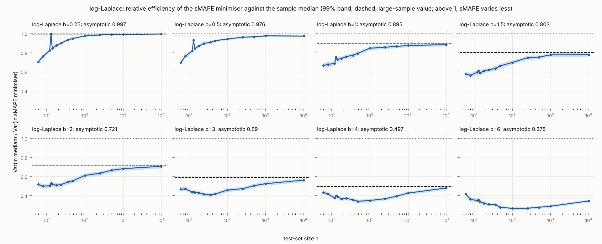
| Row | setting | relative efficiency (test-set size: 6) | relative efficiency (test-set size: 12) | relative efficiency (test-set size: 100) | relative efficiency (test-set size: 1000) | relative efficiency (test-set size: 10000) | asymptotic relative efficiency |
|---|---|---|---|---|---|---|---|
| r1 | lognormal sigma=0.25 | 0.6059 | 0.7026 | 0.8996 | 0.9662 | 0.9701 | 0.9696 |
| r2 | lognormal sigma=0.5 | 0.611 | 0.7083 | 0.8802 | 0.885 | 0.8906 | 0.8881 |
| r3 | lognormal sigma=1 | 0.6067 | 0.6555 | 0.6524 | 0.6659 | 0.6565 | 0.6601 |
| r4 | lognormal sigma=1.5 | 0.5484 | 0.5123 | 0.4595 | 0.4633 | 0.45 | 0.454 |
| r5 | lognormal sigma=2 | 0.501 | 0.4392 | 0.323 | 0.3077 | 0.3043 | 0.3073 |
| r6 | lognormal sigma=3 | 0.4381 | 0.3646 | 0.2058 | 0.1557 | 0.1513 | 0.1474 |
| r7 | lognormal sigma=4 | 0.4148 | 0.3272 | 0.1561 | 0.089 | 0.0789 | 0.0778 |
| r8 | lognormal sigma=6 | 0.3933 | 0.3027 | 0.1229 | 0.0508 | 0.0317 | 0.0279 |
| r9 | log-Laplace b=0.25 | 0.7049 | 0.8268 | 0.9769 | 0.9918 | 0.9969 | 0.9969 |
| r10 | log-Laplace b=0.5 | 0.6989 | 0.819 | 0.9448 | 0.9779 | 0.9753 | 0.9765 |
| r11 | log-Laplace b=1 | 0.667 | 0.6887 | 0.8479 | 0.8763 | 0.8853 | 0.8953 |
| r12 | log-Laplace b=1.5 | 0.5766 | 0.5947 | 0.6989 | 0.7789 | 0.7804 | 0.8035 |
| r13 | log-Laplace b=2 | 0.5179 | 0.5036 | 0.612 | 0.683 | 0.7079 | 0.7206 |
| r14 | log-Laplace b=3 | 0.4672 | 0.4365 | 0.4586 | 0.5257 | 0.5628 | 0.5902 |
| r15 | log-Laplace b=4 | 0.4353 | 0.3764 | 0.3496 | 0.4267 | 0.4803 | 0.4968 |
| r16 | log-Laplace b=6 | 0.4167 | 0.3492 | 0.2667 | 0.2896 | 0.3441 | 0.3753 |
| Row | setting | test-set size | mean of ln(sMAPE minimiser) minus ln(median) | variance of ln(sample median) | variance of ln(sMAPE minimiser) | ratio of mean squared errors about the true median |
|---|---|---|---|---|---|---|
| r1 | lognormal sigma=0.25 | 12 | 0.0008 | 0.0072 | 0.0103 | 0.7026 |
| r2 | lognormal sigma=0.25 | 1000 | 0.0000 | 0.0001 | 0.0001 | 0.9662 |
| r3 | lognormal sigma=1 | 12 | 0.0008 | 0.1159 | 0.1768 | 0.6555 |
| r4 | lognormal sigma=1 | 1000 | 0.0001 | 0.0016 | 0.0024 | 0.6659 |
| r5 | lognormal sigma=6 | 12 | 0.0021 | 4.287 | 14.17 | 0.3027 |
| r6 | lognormal sigma=6 | 1000 | -0.0209 | 0.0571 | 1.126 | 0.0507 |
| r7 | log-Laplace b=0.25 | 12 | -0.0004 | 0.0073 | 0.0088 | 0.8268 |
| r8 | log-Laplace b=0.25 | 1000 | 0.0002 | 0.0001 | 0.0001 | 0.9918 |
| r9 | log-Laplace b=1 | 12 | 0.0014 | 0.1191 | 0.173 | 0.6887 |
| r10 | log-Laplace b=1 | 1000 | 0.0003 | 0.0011 | 0.0012 | 0.8764 |
| r11 | log-Laplace b=6 | 12 | 0.0212 | 4.267 | 12.22 | 0.3492 |
| r12 | log-Laplace b=6 | 1000 | 0.003 | 0.0377 | 0.1303 | 0.2896 |
Lab runs RN10 under plan PL11. Design: Exact computation, with no sampling, of the forecasts that minimise the expected Suilin term and the expected sMAPE term (claimset-code/smape-target/msmape_targets.py, run once): by Gauss-Legendre quadrature of the density of ln y for continuous distributions (with zeros added as a point mass) and by sums for counts, minimised over forecasts f >= 0 on a grid of 0 and 4000 log-spaced points refined by golden section. Settings: away from zero, lognormal sigma 0.5 and 1, inverse Gaussian shape 10 and 100 and log-skewed sd 1 with skewness -1 and +1, all at median about 100; near zero, lognormal sigma 1 at median 1 and at median 100 with shares of zeros 0, 0.2, 0.4, 0.6 and 0.8; counts, Poisson with means 0.3, 0.5, 1, 1.5, 3 and 10. For the lognormal sigma 1 at medians 1 and 100, the share of zeros at which each measure switches to the forecast 0, by bisection. Analysis: For each setting and measure: the target, its quantile level and the expected score there; for each setting, the relative difference of the Suilin target from the sMAPE target; and the two zero thresholds. Reported as tables, with no decision rule. The plan, the run's script and its results file name the Suilin loss msMAPE, as version 2 of this paper did.
Setup: studied Suilin term, sMAPE term · cases zero-inflated outcomes, Poisson counts · procedure derived value · lens Suilin target, sMAPE target
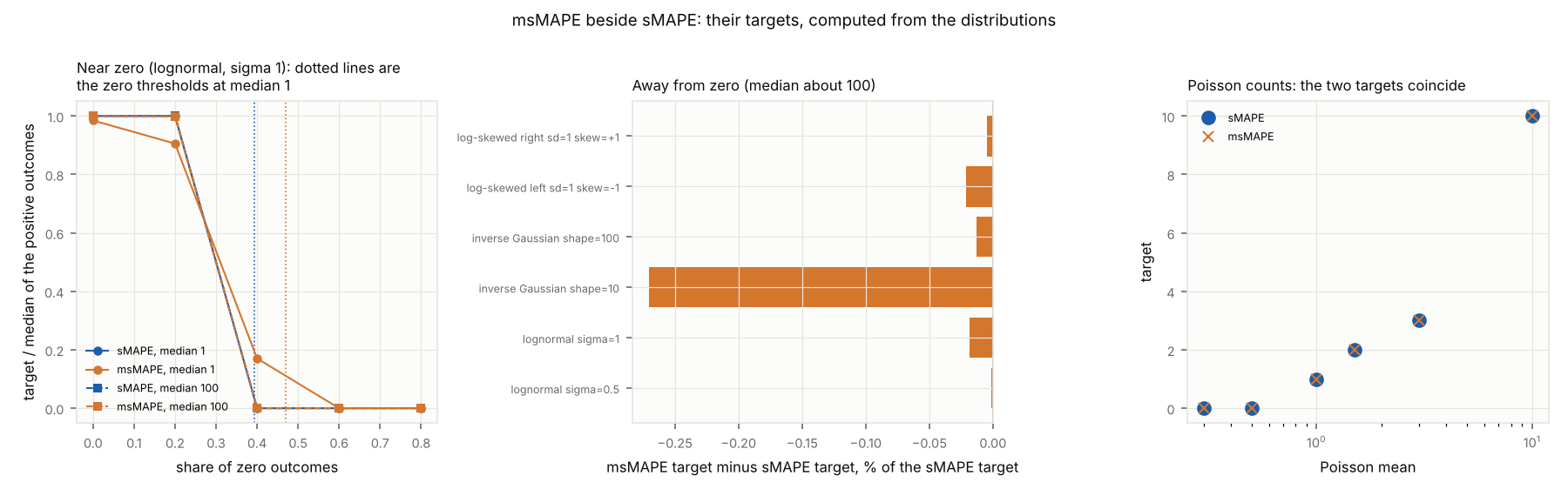
| Row | setting | target (measure: sMAPE) | target (measure: Suilin) | quantile level of the target (measure: sMAPE) | quantile level of the target (measure: Suilin) | relative difference of the Suilin target from the sMAPE target | share of zero outcomes |
|---|---|---|---|---|---|---|---|
| r1 | lognormal sigma=0.5 | 100 | 100 | 0.5 | 0.5 | 0.0000 | 0 |
| r2 | lognormal sigma=1 | 100 | 99.98 | 0.5 | 0.4999 | -0.0002 | 0 |
| r3 | inverse Gaussian shape=10 | 14.02 | 13.98 | 0.4387 | 0.438 | -0.0027 | 0 |
| r4 | inverse Gaussian shape=100 | 66.53 | 66.52 | 0.4929 | 0.4929 | -0.0001 | 0 |
| r5 | log-skewed left sd=1 skew=-1 | 128.3 | 128.2 | 0.5362 | 0.5361 | -0.0002 | 0 |
| r6 | log-skewed right sd=1 skew=+1 | 77.96 | 77.96 | 0.4638 | 0.4638 | 0.0000 | 0 |
| r7 | lognormal median=1 sigma=1 | 1 | 0.9846 | 0.5 | 0.4938 | -0.0154 | 0 |
| r8 | lognormal median=1 sigma=1 with zeros p0=0.2 | 1 | 0.9054 | 0.6 | 0.5683 | -0.0946 | 0.2 |
| r9 | lognormal median=1 sigma=1 with zeros p0=0.4 | 0 | 0.1702 | 0.4 | 0.423 | 0.4 | |
| r10 | lognormal median=1 sigma=1 with zeros p0=0.6 | 0 | 0 | 0.6 | 0.6 | 0 | 0.6 |
| r11 | lognormal median=1 sigma=1 with zeros p0=0.8 | 0 | 0 | 0.8 | 0.8 | 0 | 0.8 |
| r12 | lognormal median=100 sigma=1 | 100 | 99.98 | 0.5 | 0.4999 | -0.0002 | 0 |
| r13 | lognormal median=100 sigma=1 with zeros p0=0.2 | 100 | 99.89 | 0.6 | 0.5997 | -0.0011 | 0.2 |
| r14 | lognormal median=100 sigma=1 with zeros p0=0.4 | 0 | 0 | 0.4 | 0.4 | 0 | 0.4 |
| r15 | lognormal median=100 sigma=1 with zeros p0=0.6 | 0 | 0 | 0.6 | 0.6 | 0 | 0.6 |
| r16 | lognormal median=100 sigma=1 with zeros p0=0.8 | 0 | 0 | 0.8 | 0.8 | 0 | 0.8 |
| r17 | Poisson mean=0.3 | 0 | 0 | 0.7408 | 0.7408 | 0 | 0.7408 |
| r18 | Poisson mean=0.5 | 0 | 0 | 0.6065 | 0.6065 | 0 | 0.6065 |
| r19 | Poisson mean=1 | 1 | 1 | 0.7358 | 0.7358 | 0 | 0.3679 |
| r20 | Poisson mean=1.5 | 2 | 2 | 0.8088 | 0.8088 | 0 | 0.2231 |
| r21 | Poisson mean=3 | 3 | 3 | 0.6472 | 0.6472 | 0 | 0.0498 |
| r22 | Poisson mean=10 | 10 | 10 | 0.583 | 0.583 | 0 | 0.0000 |
| Row | setting | zero threshold (measure: sMAPE) | zero threshold (measure: Suilin) |
|---|---|---|---|
| r1 | lognormal median=1 sigma=1 | 0.394 | 0.47 |
| r2 | lognormal median=100 sigma=1 | 0.394 | 0.3937 |
Numerical checks of the formulas of the claims new or reworded in version 3 (formula checks), lab run RN13 (check_v3.py, seed 8) under the formal plan that decided C3, C4, C12, C17 and C20; every check is within the plan's tolerances. They check the formulas on concrete numbers; the proofs are the evidence for the claims. The tables are labelled by the hypotheses the run's script names: H3 (T1 and T2) checks C3; H4 (T3) checks C4; H34 (T4 and T5) checks C12; H35 (T6 and T7) checks C17; H42 (T8 and T9) checks C20. The tables of H39 (T10 to T12) and H40 (T13 to T17) check the formulas of C18 and C19, whose wording was decided after later checks (E32, E33).
Setup: studied sMAPE term, Suilin term, msMAPE term, sMAPE target, sMAPE minimiser of a test set · procedure formula checks · lens signal-to-noise ratio of a comparison, relative efficiency, weight, log error, log-MAE, MAE, RMSE
| Row | violations of the bound on the log-MAE of the sMAPE minimiser | largest excess of the minimiser's log-MAE over the median's, minus the bound |
|---|---|---|
| r1 | 0 | 0.0000 |
| Row | sum of sMAPE terms, forecast at the median, actuals 1, 1, e, e^4, e^4 | sum of sMAPE terms, forecast at 1, actuals 1, 1, e, e^4, e^4 |
|---|---|---|
| r1 | 2.735 | 2.39 |
| Row | largest difference of the weights below and above the target, over their sum |
|---|---|
| r1 | 0.0000 |
| Row | distributions with more than one local minimum | distributions where the target is not on the side of the median that carries more weight |
|---|---|---|
| r1 | 0 | 0 |
| Row | largest distance in logs between the target and the median, lognormal and log-Laplace |
|---|---|
| r1 | 0.0000 |
| Row | Suilin term of a zero forecast of a zero actual |
|---|---|
| r1 | 0 |
| Row | largest error of the identity of (a) | largest error of the identity of (b) | values of the Suilin term outside [0, 1) |
|---|---|---|---|
| r1 | 0.0000 | 0 | 0 |
| Row | nu | largest error of the identity of (a) | largest error of the identity of (b) | values of the msMAPE term outside [0, 1] | values of the msMAPE term not below 1 for actuals below nu | pairs with a count of at least 1 where the msMAPE and sMAPE terms differ |
|---|---|---|---|---|---|---|
| r1 | 0.1 | 0 | 0 | 0 | 0 | 0 |
| r2 | 0.5 | 0 | 0 | 0 | 0 | 0 |
| r3 | 1.0 | 0 | 0 | 0 | 0 | 0 |
| Row | nu | msMAPE term of a forecast of 1e-9 for a zero actual |
|---|---|---|
| r1 | 0.1 | 0.0000 |
| r2 | 0.5 | 0.0000 |
| r3 | 1.0 | 0.0000 |
| Row | error_distribution | c1 | c2 | signal-to-noise ratio of sMAPE over its large-spread formula | signal-to-noise ratio of the absolute error over its limit |
|---|---|---|---|---|---|
| r1 | normal | 0.0 | 0.5 | 0.9999 | 0.9913 |
| r2 | normal | 0.0 | 1.0 | 1 | 0.9956 |
| r3 | normal | -0.5 | 1.5 | 1.001 | 0.9966 |
| r4 | Gumbel | 0.0 | 0.5 | 0.9998 | 0.9647 |
| r5 | Gumbel | 0.0 | 1.0 | 1 | 0.9937 |
| r6 | Gumbel | -0.5 | 1.5 | 1 | 0.9967 |
| Row | error_distribution | c1 | c2 | relative spread of the absolute log error's signal-to-noise ratio over sigma = 2, 10, 50 |
|---|---|---|---|---|
| r1 | normal | 0.0 | 0.5 | 0.0000 |
| r2 | normal | 0.0 | 1.0 | 0.0000 |
| r3 | normal | -0.5 | 1.5 | 0.0000 |
| r4 | Gumbel | 0.0 | 0.5 | 0.0000 |
| r5 | Gumbel | 0.0 | 1.0 | 0.0000 |
| r6 | Gumbel | -0.5 | 1.5 | 0.0000 |
| Row | c1 | c2 | sigma | signal-to-noise ratio of the squared error over its formula, lognormal | exp(sigma^2 / 2) times the squared error's ratio, lognormal, formula |
|---|---|---|---|---|---|
| r1 | 0.0 | 0.5 | 0.5 | 1 | |
| r2 | 0.0 | 1.0 | 0.5 | 1 | |
| r3 | -0.5 | 1.5 | 0.5 | 1 | |
| r4 | 0.0 | 0.5 | 1.0 | 1 | |
| r5 | 0.0 | 1.0 | 1.0 | 1 | |
| r6 | -0.5 | 1.5 | 1.0 | 1 | |
| r7 | 0.0 | 0.5 | 2.0 | 1 | |
| r8 | 0.0 | 1.0 | 2.0 | 1 | |
| r9 | -0.5 | 1.5 | 2.0 | 1 | |
| r10 | 0.0 | 1.0 | 4.0 | 0.9907 | |
| r11 | 0.0 | 1.0 | 6.0 | 1 |
| Row | distributions compared with the asymptotic values recorded by RN7 |
|---|---|
| r1 | 16 |
| Row | distributions where A is not below 2 g at the median | largest difference from the asymptotic values recorded by RN7 |
|---|---|---|
| r1 | 0 | 0.0001 |
| Row | family | spread | large-sample relative efficiency, formula |
|---|---|---|---|
| r1 | lognormal | 0.25 | 0.9696 |
| r2 | lognormal | 0.5 | 0.8881 |
| r3 | lognormal | 1.0 | 0.6601 |
| r4 | lognormal | 1.5 | 0.454 |
| r5 | lognormal | 2.0 | 0.3073 |
| r6 | lognormal | 3.0 | 0.1474 |
| r7 | lognormal | 4.0 | 0.0778 |
| r8 | lognormal | 6.0 | 0.0279 |
| r9 | log-Laplace | 0.25 | 0.9969 |
| r10 | log-Laplace | 0.5 | 0.9765 |
| r11 | log-Laplace | 1.0 | 0.8953 |
| r12 | log-Laplace | 1.5 | 0.8036 |
| r13 | log-Laplace | 2.0 | 0.7207 |
| r14 | log-Laplace | 3.0 | 0.5903 |
| r15 | log-Laplace | 4.0 | 0.4969 |
| r16 | log-Laplace | 6.0 | 0.3755 |
| Row | family | distance of the large-sample relative efficiency from 1 at spread 0.01 |
|---|---|---|
| r1 | lognormal | 0.0001 |
| r2 | log-Laplace | 0.0000 |
| Row | large-sample relative efficiency times sigma^3 over 6 (ln 2)^2 sqrt(2 pi), lognormal | large-sample relative efficiency times b over 3, log-Laplace |
|---|---|---|
| r1 | 0.9998 | 0.9906 |
Numerical checks of the formulas of C18 (formula checks), lab run RN18 (check_h39.py) under the formal plan that decided C18; every check is within the plan's tolerances. They check the formulas on concrete numbers; the proof is the evidence for the claim. The run's script labels the checks H39, the record's first wording of C18; the formulas are those of C18.
Setup: studied sMAPE term · procedure formula checks · lens signal-to-noise ratio of a comparison, log-MAE, MAE, RMSE
| Row | error_distribution | c1 | c2 | sigma | distance of sMAPE's signal-to-noise ratio over its large-spread formula from 1 | distance of the absolute error's signal-to-noise ratio over its limit from 1 |
|---|---|---|---|---|---|---|
| r1 | normal | 0.0 | 0.5 | 200 | 0.0001 | 0.0087 |
| r2 | normal | 0.0 | 0.5 | 2000 | 0.0000 | 0.0009 |
| r3 | normal | 0.0 | 1.0 | 200 | 0.0004 | 0.0044 |
| r4 | normal | 0.0 | 1.0 | 2000 | 0.0000 | 0.0004 |
| r5 | normal | -0.5 | 1.5 | 200 | 0.0012 | 0.0034 |
| r6 | normal | -0.5 | 1.5 | 2000 | 0.0001 | 0.0003 |
| r7 | Gumbel | 0.0 | 0.5 | 200 | 0.0002 | 0.0353 |
| r8 | Gumbel | 0.0 | 0.5 | 2000 | 0.0000 | 0.0035 |
| r9 | Gumbel | 0.0 | 1.0 | 200 | 0.0002 | 0.0063 |
| r10 | Gumbel | 0.0 | 1.0 | 2000 | 0.0000 | 0.0006 |
| r11 | Gumbel | -0.5 | 1.5 | 200 | 0.0004 | 0.0033 |
| r12 | Gumbel | -0.5 | 1.5 | 2000 | 0.0000 | 0.0003 |
| Row | error_distribution | c1 | c2 | relative spread of the absolute log error's signal-to-noise ratio over sigma = 2, 10, 50 |
|---|---|---|---|---|
| r1 | normal | 0.0 | 0.5 | 0.0000 |
| r2 | normal | 0.0 | 1.0 | 0.0000 |
| r3 | normal | -0.5 | 1.5 | 0.0000 |
| r4 | Gumbel | 0.0 | 0.5 | 0.0000 |
| r5 | Gumbel | 0.0 | 1.0 | 0.0000 |
| r6 | Gumbel | -0.5 | 1.5 | 0.0000 |
| Row | c1 | c2 | sigma | distance of the squared error's signal-to-noise ratio over its formula from 1, lognormal | distance of exp(sigma^2 / 2) times the squared error's ratio from 1, lognormal, formula |
|---|---|---|---|---|---|
| r1 | 0.0 | 0.5 | 0.5 | 0.0000 | |
| r2 | 0.0 | 1.0 | 0.5 | 0.0000 | |
| r3 | -0.5 | 1.5 | 0.5 | 0.0000 | |
| r4 | 0.0 | 0.5 | 1.0 | 0.0000 | |
| r5 | 0.0 | 1.0 | 1.0 | 0.0000 | |
| r6 | -0.5 | 1.5 | 1.0 | 0.0000 | |
| r7 | 0.0 | 0.5 | 2.0 | 0.0000 | |
| r8 | 0.0 | 1.0 | 2.0 | 0.0000 | |
| r9 | -0.5 | 1.5 | 2.0 | 0.0000 | |
| r10 | 0.0 | 1.0 | 4.0 | 0.0093 | |
| r11 | 0.0 | 1.0 | 6.0 | 0.0000 | |
| r12 | 0.0 | 1.0 | 8.0 | 0.0000 |
Numerical checks of the formulas of C19 (formula checks), lab run RN16 (check_corrected.py, seed 8) under the formal plan that decided C19; every check is within the plan's tolerances. They check the formulas on concrete numbers; the proof is the evidence for the claim. The run's script labels the checks by the record's first wordings: H40 (T4 to T7 and the result R1) checks C19; H39 (T1 to T3) checks the formulas of C18, which the same plan tested in an earlier wording.
Setup: studied sMAPE term, sMAPE minimiser of a test set · procedure formula checks · lens signal-to-noise ratio of a comparison, relative efficiency, log-MAE, MAE, RMSE
- R1 distributions compared with the asymptotic values recorded by RN7 = 16 (hypothesis: H40)
| Row | error_distribution | c1 | c2 | sigma | distance of sMAPE's signal-to-noise ratio over its large-spread formula from 1 | distance of the absolute error's signal-to-noise ratio over its limit from 1 |
|---|---|---|---|---|---|---|
| r1 | normal | 0.0 | 0.5 | 200 | 0.0001 | 0.0087 |
| r2 | normal | 0.0 | 0.5 | 2000 | 0.0000 | 0.0009 |
| r3 | normal | 0.0 | 1.0 | 200 | 0.0004 | 0.0044 |
| r4 | normal | 0.0 | 1.0 | 2000 | 0.0000 | 0.0004 |
| r5 | normal | -0.5 | 1.5 | 200 | 0.0012 | 0.0034 |
| r6 | normal | -0.5 | 1.5 | 2000 | 0.0001 | 0.0003 |
| r7 | Gumbel | 0.0 | 0.5 | 200 | 0.0002 | 0.0353 |
| r8 | Gumbel | 0.0 | 0.5 | 2000 | 0.0000 | 0.0035 |
| r9 | Gumbel | 0.0 | 1.0 | 200 | 0.0002 | 0.0063 |
| r10 | Gumbel | 0.0 | 1.0 | 2000 | 0.0000 | 0.0006 |
| r11 | Gumbel | -0.5 | 1.5 | 200 | 0.0004 | 0.0033 |
| r12 | Gumbel | -0.5 | 1.5 | 2000 | 0.0000 | 0.0003 |
| Row | error_distribution | c1 | c2 | relative spread of the absolute log error's signal-to-noise ratio over sigma = 2, 10, 50 |
|---|---|---|---|---|
| r1 | normal | 0.0 | 0.5 | 0.0000 |
| r2 | normal | 0.0 | 1.0 | 0.0000 |
| r3 | normal | -0.5 | 1.5 | 0.0000 |
| r4 | Gumbel | 0.0 | 0.5 | 0.0000 |
| r5 | Gumbel | 0.0 | 1.0 | 0.0000 |
| r6 | Gumbel | -0.5 | 1.5 | 0.0000 |
| Row | c1 | c2 | sigma | distance of the squared error's signal-to-noise ratio over its formula from 1, lognormal | distance of exp(sigma^2 / 2) times the squared error's ratio from 1, lognormal, formula |
|---|---|---|---|---|---|
| r1 | 0.0 | 0.5 | 0.5 | 0.0000 | |
| r2 | 0.0 | 1.0 | 0.5 | 0.0000 | |
| r3 | -0.5 | 1.5 | 0.5 | 0.0000 | |
| r4 | 0.0 | 0.5 | 1.0 | 0.0000 | |
| r5 | 0.0 | 1.0 | 1.0 | 0.0000 | |
| r6 | -0.5 | 1.5 | 1.0 | 0.0000 | |
| r7 | 0.0 | 0.5 | 2.0 | 0.0000 | |
| r8 | 0.0 | 1.0 | 2.0 | 0.0000 | |
| r9 | -0.5 | 1.5 | 2.0 | 0.0000 | |
| r10 | 0.0 | 1.0 | 4.0 | 0.0093 | |
| r11 | 0.0 | 1.0 | 6.0 | 0.0000 | |
| r12 | 0.0 | 1.0 | 8.0 | 0.0000 |
| Row | family | spread | large-sample relative efficiency, formula |
|---|---|---|---|
| r1 | lognormal | 0.25 | 0.9696 |
| r2 | lognormal | 0.5 | 0.8881 |
| r3 | lognormal | 1.0 | 0.6601 |
| r4 | lognormal | 1.5 | 0.454 |
| r5 | lognormal | 2.0 | 0.3073 |
| r6 | lognormal | 3.0 | 0.1474 |
| r7 | lognormal | 4.0 | 0.0778 |
| r8 | lognormal | 6.0 | 0.0279 |
| r9 | log-Laplace | 0.25 | 0.9969 |
| r10 | log-Laplace | 0.5 | 0.9765 |
| r11 | log-Laplace | 1.0 | 0.8953 |
| r12 | log-Laplace | 1.5 | 0.8036 |
| r13 | log-Laplace | 2.0 | 0.7207 |
| r14 | log-Laplace | 3.0 | 0.5903 |
| r15 | log-Laplace | 4.0 | 0.4969 |
| r16 | log-Laplace | 6.0 | 0.3755 |
| Row | family | distance of the large-sample relative efficiency from 1 at spread 0.01 |
|---|---|---|
| r1 | lognormal | 0.0001 |
| r2 | log-Laplace | 0.0000 |
| Row | distributions where A is not below 2 g at the median | largest difference from the asymptotic values recorded by RN7 |
|---|---|---|
| r1 | 0 | 0.0001 |
| Row | large-sample relative efficiency times sigma^3 over 6 (ln 2)^2 sqrt(2 pi), lognormal | large-sample relative efficiency times b over 3, log-Laplace |
|---|---|---|
| r1 | 0.9998 | 0.9906 |
Lab runs RN15 under plan PL14. Design: Which forecast does msMAPE reward on intermittent demand, beside sMAPE and the Suilin loss? One run of python3 claimset-code/smape-target/msmape_intermittent.py --seed 9, in two parts, for five measures: sMAPE, msMAPE with nu = 0.1, 0.5 and 1, and the Suilin loss, on the 14 intermittent demand settings. (1) Exact, with no sampling: the forecast that minimises the expected term of each measure (sums for counts; Gauss-Legendre quadrature of the density of ln y with the zeros as a point mass for the lognormal settings), minimised over forecasts f >= 0 on a grid of 0, the integers and 4000 log-spaced points, refined by golden section; and, for the lognormal demand sizes, the share of zeros at which each measure switches to the forecast 0, by bisection. (2) Simulated: test sets of n = 12, 52 and 365 independent actuals (a year of months, of weeks and of days), 2000 test sets per setting and n; in each test set, the forecast with the lowest value of each measure, searched over 0, the test set's own values and a grid (step 0.05 up to the largest value plus 1 for counts; 400 log-spaced points for the lognormal settings). Analysis: Part 1, per setting and measure: the target, its quantile level and the expected score there, beside the setting's share of zeros, median, mode and mean, so that the functional the target coincides with can be read; per measure, the zero threshold. Part 2, per setting, measure and n: the share of test sets whose minimiser is 0, the share whose minimiser is the exact target of part 1 (counts), and the median of the minimisers. Reported as tables and one figure (the targets against the share of zeros, a panel per measure); no test is made and no threshold is set. The figure as drawn (A56) has a panel per family of settings and a line per measure.
Setup: studied msMAPE term, sMAPE term, Suilin term · cases intermittent demand settings · procedure derived value · lens msMAPE target, sMAPE target, Suilin target
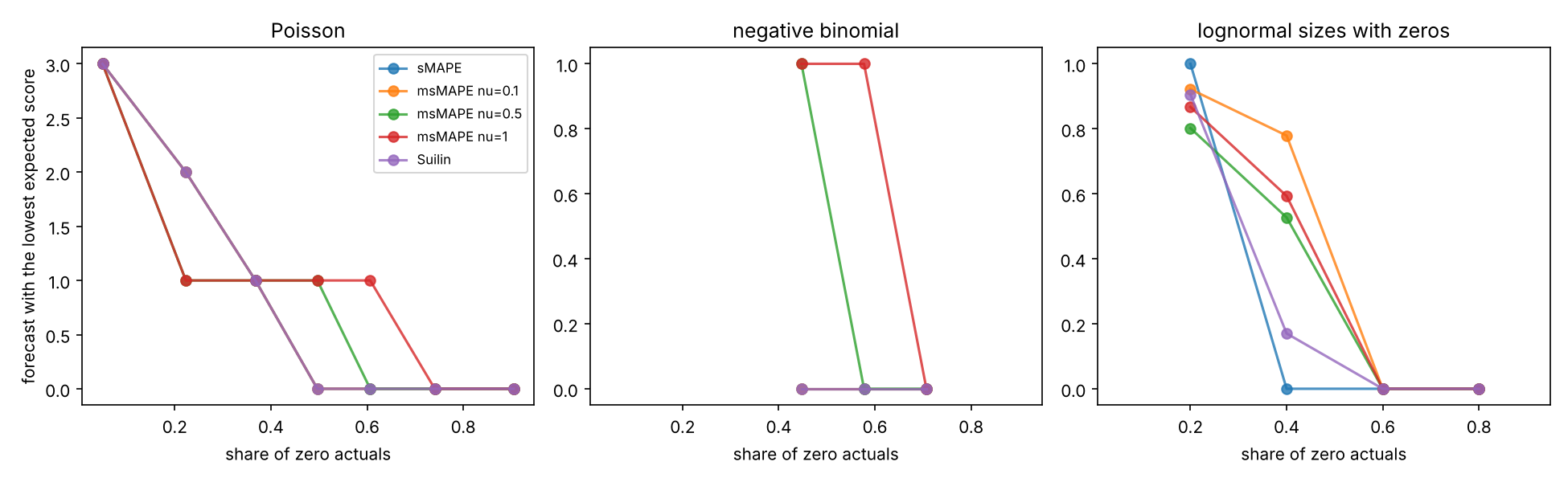
| Row | setting | share of zero outcomes | median of the outcomes | mode of the outcomes | mean of the outcomes | target (measure: sMAPE) | target (measure: msMAPE nu=0.1) | target (measure: msMAPE nu=0.5) | target (measure: msMAPE nu=1) | target (measure: Suilin) |
|---|---|---|---|---|---|---|---|---|---|---|
| r1 | Poisson mean=0.1 | 0.9048 | 0 | 0 | 0.1 | 0 | 0 | 0 | 0 | 0 |
| r2 | Poisson mean=0.3 | 0.7408 | 0 | 0 | 0.3 | 0 | 0 | 0 | 0 | 0 |
| r3 | Poisson mean=0.5 | 0.6065 | 0 | 0 | 0.5 | 0 | 0 | 0 | 1 | 0 |
| r4 | Poisson mean=0.7 | 0.4966 | 1 | 0 | 0.7 | 0 | 0 | 1 | 1 | 0 |
| r5 | Poisson mean=1 | 0.3679 | 1 | 0 | 1 | 1 | 1 | 1 | 1 | 1 |
| r6 | Poisson mean=1.5 | 0.2231 | 1 | 1 | 1.5 | 2 | 2 | 1 | 1 | 2 |
| r7 | Poisson mean=3 | 0.0498 | 3 | 2 | 3 | 3 | 3 | 3 | 3 | 3 |
| r8 | negative binomial mean=0.5 size=0.5 | 0.7071 | 0 | 0 | 0.5 | 0 | 0 | 0 | 0 | 0 |
| r9 | negative binomial mean=1 size=0.5 | 0.5774 | 0 | 0 | 1 | 0 | 0 | 0 | 1 | 0 |
| r10 | negative binomial mean=2 size=0.5 | 0.4472 | 1 | 0 | 2 | 0 | 0 | 1 | 1 | 0 |
| r11 | lognormal sizes with zeros p0=0.2 | 0.2 | 0.7271 | 1.319 | 1 | 0.922 | 0.8021 | 0.8672 | 0.9054 | |
| r12 | lognormal sizes with zeros p0=0.4 | 0.4 | 0.3801 | 0.9892 | 0 | 0.7791 | 0.5271 | 0.5932 | 0.1702 | |
| r13 | lognormal sizes with zeros p0=0.6 | 0.6 | 0 | 0.6595 | 0 | 0 | 0 | 0 | 0 | |
| r14 | lognormal sizes with zeros p0=0.8 | 0.8 | 0 | 0.3297 | 0 | 0 | 0 | 0 | 0 |
| Row | setting | zero threshold (measure: sMAPE) | zero threshold (measure: msMAPE nu=0.1) | zero threshold (measure: msMAPE nu=0.5) | zero threshold (measure: msMAPE nu=1) | zero threshold (measure: Suilin) |
|---|---|---|---|---|---|---|
| r1 | lognormal sizes with zeros | 0.394 | 0.4191 | 0.5192 | 0.5647 | 0.47 |
| Row | setting | quantile level of the target (measure: sMAPE) | quantile level of the target (measure: msMAPE nu=0.1) | quantile level of the target (measure: msMAPE nu=0.5) | quantile level of the target (measure: msMAPE nu=1) | quantile level of the target (measure: Suilin) | expected score at the target (measure: sMAPE) | expected score at the target (measure: msMAPE nu=0.1) | expected score at the target (measure: msMAPE nu=0.5) | expected score at the target (measure: msMAPE nu=1) | expected score at the target (measure: Suilin) |
|---|---|---|---|---|---|---|---|---|---|---|---|
| r1 | Poisson mean=0.1 | 0.9048 | 0.9048 | 0.9048 | 0.9048 | 0.9048 | 19.03 | 19.03 | 19.03 | 19.03 | 17.34 |
| r2 | Poisson mean=0.3 | 0.7408 | 0.7408 | 0.7408 | 0.7408 | 0.7408 | 51.84 | 51.84 | 51.84 | 51.84 | 47.46 |
| r3 | Poisson mean=0.5 | 0.6065 | 0.6065 | 0.6065 | 0.9098 | 0.6065 | 78.69 | 78.69 | 78.69 | 67.18 | 72.37 |
| r4 | Poisson mean=0.7 | 0.4966 | 0.4966 | 0.8442 | 0.8442 | 0.4966 | 100.7 | 100.7 | 77.86 | 61.31 | 92.99 |
| r5 | Poisson mean=1 | 0.7358 | 0.7358 | 0.7358 | 0.7358 | 0.7358 | 94.3 | 87.61 | 69.78 | 57.52 | 87.03 |
| r6 | Poisson mean=1.5 | 0.8088 | 0.8088 | 0.5578 | 0.5578 | 0.8088 | 76.77 | 74.64 | 67.21 | 59.77 | 73.75 |
| r7 | Poisson mean=3 | 0.6472 | 0.6472 | 0.6472 | 0.6472 | 0.6472 | 49.91 | 49.59 | 48.49 | 47.42 | 48.86 |
| r8 | negative binomial mean=0.5 size=0.5 | 0.7071 | 0.7071 | 0.7071 | 0.7071 | 0.7071 | 58.58 | 58.58 | 58.58 | 58.58 | 54.46 |
| r9 | negative binomial mean=1 size=0.5 | 0.5774 | 0.5774 | 0.5774 | 0.7698 | 0.5774 | 84.53 | 84.53 | 84.53 | 80.38 | 79.46 |
| r10 | negative binomial mean=2 size=0.5 | 0.4472 | 0.4472 | 0.6261 | 0.6261 | 0.4472 | 110.6 | 110.6 | 101.9 | 86.95 | 105.2 |
| r11 | lognormal sizes with zeros p0=0.2 | 0.6 | 0.5741 | 0.5302 | 0.5547 | 0.5683 | 95.95 | 92.15 | 78.37 | 66.53 | 89.49 |
| r12 | lognormal sizes with zeros p0=0.4 | 0.4 | 0.6409 | 0.5566 | 0.5805 | 0.423 | 120 | 113.9 | 87.15 | 70.9 | 94.45 |
| r13 | lognormal sizes with zeros p0=0.6 | 0.6 | 0.6 | 0.6 | 0.6 | 0.6 | 80 | 79.78 | 72.4 | 60.93 | 65.9 |
| r14 | lognormal sizes with zeros p0=0.8 | 0.8 | 0.8 | 0.8 | 0.8 | 0.8 | 40 | 39.89 | 36.2 | 30.46 | 32.95 |
| Row | setting | n | share of test sets whose minimiser is 0 (measure: sMAPE) | share of test sets whose minimiser is 0 (measure: msMAPE nu=0.1) | share of test sets whose minimiser is 0 (measure: msMAPE nu=0.5) | share of test sets whose minimiser is 0 (measure: msMAPE nu=1) | share of test sets whose minimiser is 0 (measure: Suilin) |
|---|---|---|---|---|---|---|---|
| r1 | Poisson mean=0.1 | 12 | 1 | 0.9995 | 0.996 | 0.975 | 1 |
| r2 | Poisson mean=0.1 | 52 | 1 | 1 | 1 | 1 | 1 |
| r3 | Poisson mean=0.1 | 365 | 1 | 1 | 1 | 1 | 1 |
| r4 | Poisson mean=0.3 | 12 | 0.979 | 0.937 | 0.831 | 0.7145 | 0.979 |
| r5 | Poisson mean=0.3 | 52 | 1 | 1 | 0.9915 | 0.9155 | 1 |
| r6 | Poisson mean=0.3 | 365 | 1 | 1 | 1 | 0.9995 | 1 |
| r7 | Poisson mean=0.5 | 12 | 0.848 | 0.7525 | 0.539 | 0.378 | 0.848 |
| r8 | Poisson mean=0.5 | 52 | 0.9685 | 0.923 | 0.6515 | 0.288 | 0.966 |
| r9 | Poisson mean=0.5 | 365 | 1 | 1 | 0.8445 | 0.067 | 1 |
| r10 | Poisson mean=0.7 | 12 | 0.6045 | 0.515 | 0.2915 | 0.1555 | 0.6045 |
| r11 | Poisson mean=0.7 | 52 | 0.6575 | 0.523 | 0.1525 | 0.0265 | 0.6455 |
| r12 | Poisson mean=0.7 | 365 | 0.844 | 0.56 | 0.0025 | 0 | 0.8295 |
| r13 | Poisson mean=1 | 12 | 0.256 | 0.2265 | 0.0895 | 0.037 | 0.256 |
| r14 | Poisson mean=1 | 52 | 0.1015 | 0.051 | 0.003 | 0 | 0.1 |
| r15 | Poisson mean=1 | 365 | 0 | 0 | 0 | 0 | 0 |
| r16 | Poisson mean=1.5 | 12 | 0.0325 | 0.03 | 0.0075 | 0.002 | 0.0325 |
| r17 | Poisson mean=1.5 | 52 | 0.0005 | 0.0005 | 0 | 0 | 0.0005 |
| r18 | Poisson mean=1.5 | 365 | 0 | 0 | 0 | 0 | 0 |
| r19 | Poisson mean=3 | 12 | 0 | 0 | 0 | 0 | 0 |
| r20 | Poisson mean=3 | 52 | 0 | 0 | 0 | 0 | 0 |
| r21 | Poisson mean=3 | 365 | 0 | 0 | 0 | 0 | 0 |
| r22 | negative binomial mean=0.5 size=0.5 | 12 | 0.971 | 0.952 | 0.857 | 0.721 | 0.9705 |
| r23 | negative binomial mean=0.5 size=0.5 | 52 | 1 | 1 | 0.9895 | 0.9095 | 1 |
| r24 | negative binomial mean=0.5 size=0.5 | 365 | 1 | 1 | 1 | 1 | 1 |
| r25 | negative binomial mean=1 size=0.5 | 12 | 0.8035 | 0.78 | 0.621 | 0.4435 | 0.808 |
| r26 | negative binomial mean=1 size=0.5 | 52 | 0.975 | 0.9625 | 0.7675 | 0.405 | 0.974 |
| r27 | negative binomial mean=1 size=0.5 | 365 | 1 | 1 | 0.975 | 0.256 | 1 |
| r28 | negative binomial mean=2 size=0.5 | 12 | 0.567 | 0.5265 | 0.384 | 0.2405 | 0.5765 |
| r29 | negative binomial mean=2 size=0.5 | 52 | 0.707 | 0.635 | 0.3055 | 0.068 | 0.7255 |
| r30 | negative binomial mean=2 size=0.5 | 365 | 0.932 | 0.8475 | 0.1115 | 0 | 0.9475 |
| r31 | lognormal sizes with zeros p0=0.2 | 12 | 0.046 | 0.026 | 0.0055 | 0.002 | 0.016 |
| r32 | lognormal sizes with zeros p0=0.2 | 52 | 0 | 0 | 0 | 0 | 0 |
| r33 | lognormal sizes with zeros p0=0.2 | 365 | 0 | 0 | 0 | 0 | 0 |
| r34 | lognormal sizes with zeros p0=0.4 | 12 | 0.4655 | 0.374 | 0.1735 | 0.119 | 0.303 |
| r35 | lognormal sizes with zeros p0=0.4 | 52 | 0.5235 | 0.36 | 0.045 | 0.012 | 0.172 |
| r36 | lognormal sizes with zeros p0=0.4 | 365 | 0.5665 | 0.207 | 0 | 0 | 0.004 |
| r37 | lognormal sizes with zeros p0=0.6 | 12 | 0.896 | 0.8565 | 0.663 | 0.5805 | 0.8055 |
| r38 | lognormal sizes with zeros p0=0.6 | 52 | 0.9975 | 0.993 | 0.844 | 0.6765 | 0.9705 |
| r39 | lognormal sizes with zeros p0=0.6 | 365 | 1 | 1 | 0.999 | 0.892 | 1 |
| r40 | lognormal sizes with zeros p0=0.8 | 12 | 0.9975 | 0.9955 | 0.9725 | 0.959 | 0.991 |
| r41 | lognormal sizes with zeros p0=0.8 | 52 | 1 | 1 | 1 | 0.9995 | 1 |
| r42 | lognormal sizes with zeros p0=0.8 | 365 | 1 | 1 | 1 | 1 | 1 |
| Row | setting | n | share of test sets whose minimiser is the target (measure: sMAPE) | share of test sets whose minimiser is the target (measure: msMAPE nu=0.1) | share of test sets whose minimiser is the target (measure: msMAPE nu=0.5) | share of test sets whose minimiser is the target (measure: msMAPE nu=1) | share of test sets whose minimiser is the target (measure: Suilin) |
|---|---|---|---|---|---|---|---|
| r1 | Poisson mean=0.1 | 12 | 1 | 0.9995 | 0.996 | 0.975 | 1 |
| r2 | Poisson mean=0.1 | 52 | 1 | 1 | 1 | 1 | 1 |
| r3 | Poisson mean=0.1 | 365 | 1 | 1 | 1 | 1 | 1 |
| r4 | Poisson mean=0.3 | 12 | 0.979 | 0.937 | 0.831 | 0.7145 | 0.979 |
| r5 | Poisson mean=0.3 | 52 | 1 | 1 | 0.9915 | 0.9155 | 1 |
| r6 | Poisson mean=0.3 | 365 | 1 | 1 | 1 | 0.9995 | 1 |
| r7 | Poisson mean=0.5 | 12 | 0.848 | 0.7525 | 0.539 | 0.547 | 0.848 |
| r8 | Poisson mean=0.5 | 52 | 0.9685 | 0.923 | 0.6515 | 0.712 | 0.966 |
| r9 | Poisson mean=0.5 | 365 | 1 | 1 | 0.8445 | 0.933 | 1 |
| r10 | Poisson mean=0.7 | 12 | 0.6045 | 0.515 | 0.691 | 0.8035 | 0.6045 |
| r11 | Poisson mean=0.7 | 52 | 0.6575 | 0.523 | 0.8475 | 0.9735 | 0.6455 |
| r12 | Poisson mean=0.7 | 365 | 0.844 | 0.56 | 0.9975 | 1 | 0.8295 |
| r13 | Poisson mean=1 | 12 | 0.5335 | 0.5665 | 0.775 | 0.8565 | 0.537 |
| r14 | Poisson mean=1 | 52 | 0.7705 | 0.8855 | 0.9825 | 0.993 | 0.8415 |
| r15 | Poisson mean=1 | 365 | 0.9985 | 1 | 1 | 1 | 1 |
| r16 | Poisson mean=1.5 | 12 | 0.5675 | 0.569 | 0.457 | 0.501 | 0.5685 |
| r17 | Poisson mean=1.5 | 52 | 0.7395 | 0.657 | 0.5585 | 0.6325 | 0.6565 |
| r18 | Poisson mean=1.5 | 365 | 0.9635 | 0.867 | 0.5965 | 0.762 | 0.8665 |
| r19 | Poisson mean=3 | 12 | 0.552 | 0.5475 | 0.5515 | 0.554 | 0.548 |
| r20 | Poisson mean=3 | 52 | 0.8905 | 0.888 | 0.884 | 0.8795 | 0.889 |
| r21 | Poisson mean=3 | 365 | 1 | 1 | 1 | 1 | 1 |
| r22 | negative binomial mean=0.5 size=0.5 | 12 | 0.971 | 0.952 | 0.857 | 0.721 | 0.9705 |
| r23 | negative binomial mean=0.5 size=0.5 | 52 | 1 | 1 | 0.9895 | 0.9095 | 1 |
| r24 | negative binomial mean=0.5 size=0.5 | 365 | 1 | 1 | 1 | 1 | 1 |
| r25 | negative binomial mean=1 size=0.5 | 12 | 0.8035 | 0.78 | 0.621 | 0.471 | 0.808 |
| r26 | negative binomial mean=1 size=0.5 | 52 | 0.975 | 0.9625 | 0.7675 | 0.592 | 0.974 |
| r27 | negative binomial mean=1 size=0.5 | 365 | 1 | 1 | 0.975 | 0.744 | 1 |
| r28 | negative binomial mean=2 size=0.5 | 12 | 0.567 | 0.5265 | 0.3345 | 0.4825 | 0.5765 |
| r29 | negative binomial mean=2 size=0.5 | 52 | 0.707 | 0.635 | 0.473 | 0.782 | 0.7255 |
| r30 | negative binomial mean=2 size=0.5 | 365 | 0.932 | 0.8475 | 0.855 | 0.998 | 0.9475 |
| Row | setting | n | median of the test-set minimisers (measure: sMAPE) | median of the test-set minimisers (measure: msMAPE nu=0.1) | median of the test-set minimisers (measure: msMAPE nu=0.5) | median of the test-set minimisers (measure: msMAPE nu=1) | median of the test-set minimisers (measure: Suilin) |
|---|---|---|---|---|---|---|---|
| r1 | Poisson mean=0.1 | 12 | 0 | 0 | 0 | 0 | 0 |
| r2 | Poisson mean=0.1 | 52 | 0 | 0 | 0 | 0 | 0 |
| r3 | Poisson mean=0.1 | 365 | 0 | 0 | 0 | 0 | 0 |
| r4 | Poisson mean=0.3 | 12 | 0 | 0 | 0 | 0 | 0 |
| r5 | Poisson mean=0.3 | 52 | 0 | 0 | 0 | 0 | 0 |
| r6 | Poisson mean=0.3 | 365 | 0 | 0 | 0 | 0 | 0 |
| r7 | Poisson mean=0.5 | 12 | 0 | 0 | 0 | 1 | 0 |
| r8 | Poisson mean=0.5 | 52 | 0 | 0 | 0 | 1 | 0 |
| r9 | Poisson mean=0.5 | 365 | 0 | 0 | 0 | 1 | 0 |
| r10 | Poisson mean=0.7 | 12 | 0 | 0 | 1 | 1 | 0 |
| r11 | Poisson mean=0.7 | 52 | 0 | 0 | 1 | 1 | 0 |
| r12 | Poisson mean=0.7 | 365 | 0 | 0 | 1 | 1 | 0 |
| r13 | Poisson mean=1 | 12 | 1 | 1 | 1 | 1 | 1 |
| r14 | Poisson mean=1 | 52 | 1 | 1 | 1 | 1 | 1 |
| r15 | Poisson mean=1 | 365 | 1 | 1 | 1 | 1 | 1 |
| r16 | Poisson mean=1.5 | 12 | 2 | 2 | 2 | 1 | 2 |
| r17 | Poisson mean=1.5 | 52 | 2 | 2 | 1 | 1 | 2 |
| r18 | Poisson mean=1.5 | 365 | 2 | 2 | 1 | 1 | 2 |
| r19 | Poisson mean=3 | 12 | 3 | 3 | 3 | 3 | 3 |
| r20 | Poisson mean=3 | 52 | 3 | 3 | 3 | 3 | 3 |
| r21 | Poisson mean=3 | 365 | 3 | 3 | 3 | 3 | 3 |
| r22 | negative binomial mean=0.5 size=0.5 | 12 | 0 | 0 | 0 | 0 | 0 |
| r23 | negative binomial mean=0.5 size=0.5 | 52 | 0 | 0 | 0 | 0 | 0 |
| r24 | negative binomial mean=0.5 size=0.5 | 365 | 0 | 0 | 0 | 0 | 0 |
| r25 | negative binomial mean=1 size=0.5 | 12 | 0 | 0 | 0 | 1 | 0 |
| r26 | negative binomial mean=1 size=0.5 | 52 | 0 | 0 | 0 | 1 | 0 |
| r27 | negative binomial mean=1 size=0.5 | 365 | 0 | 0 | 0 | 1 | 0 |
| r28 | negative binomial mean=2 size=0.5 | 12 | 0 | 0 | 1 | 1 | 0 |
| r29 | negative binomial mean=2 size=0.5 | 52 | 0 | 0 | 1 | 1 | 0 |
| r30 | negative binomial mean=2 size=0.5 | 365 | 0 | 0 | 1 | 1 | 0 |
| r31 | lognormal sizes with zeros p0=0.2 | 12 | 0.9791 | 0.917 | 0.8181 | 0.8745 | 0.8357 |
| r32 | lognormal sizes with zeros p0=0.2 | 52 | 1.003 | 0.9223 | 0.7943 | 0.8633 | 0.8825 |
| r33 | lognormal sizes with zeros p0=0.2 | 365 | 1.003 | 0.9257 | 0.8006 | 0.8684 | 0.907 |
| r34 | lognormal sizes with zeros p0=0.4 | 12 | 0.4646 | 0.5008 | 0.5196 | 0.6003 | 0.1931 |
| r35 | lognormal sizes with zeros p0=0.4 | 52 | 0 | 0.63 | 0.5224 | 0.5913 | 0.1681 |
| r36 | lognormal sizes with zeros p0=0.4 | 365 | 0 | 0.7535 | 0.5278 | 0.5938 | 0.1719 |
| r37 | lognormal sizes with zeros p0=0.6 | 12 | 0 | 0 | 0 | 0 | 0 |
| r38 | lognormal sizes with zeros p0=0.6 | 52 | 0 | 0 | 0 | 0 | 0 |
| r39 | lognormal sizes with zeros p0=0.6 | 365 | 0 | 0 | 0 | 0 | 0 |
| r40 | lognormal sizes with zeros p0=0.8 | 12 | 0 | 0 | 0 | 0 | 0 |
| r41 | lognormal sizes with zeros p0=0.8 | 52 | 0 | 0 | 0 | 0 | 0 |
| r42 | lognormal sizes with zeros p0=0.8 | 365 | 0 | 0 | 0 | 0 | 0 |
Proof of C1 (section H1 of the proof document A1, rendered in A2). Only the ratio of the actual to the forecast matters, not their size.
Foundation: Kolmogorov probability axioms and real analysis
- Since and are positive, . So . (algebra; from D1)
- Dividing the numerator and the denominator by gives . Since , . And . (algebra; from S1)
- So . The contribution depends only on the ratio of actual to forecast. (conclusion; from S2)
Proof of C2 (section H2 of the proof document A1, rendered in A2). sMAPE is symmetric in ratios. It favours a high forecast only when errors are compared in absolute terms.
Foundation: Kolmogorov probability axioms and real analysis
- By C1, . Replacing by gives . Multiplying the numerator and the denominator by gives , the same value. (algebra; from C1)
- The forecast has , and has . By step 1 they score the same. This is (a). (algebra; from S1)
- The forecasts and are both away from , so both numerators are . The denominators are and . The larger denominator gives the smaller value. This is (b). (algebra; from S2)
- So sMAPE treats a forecast times too high and one times too low alike. It favours the high forecast only when the two are equally wrong in absolute terms. (conclusion; from S3)
Proof of C3 (section H3 of the proof document A1, rendered in A2). sMAPE measures the error on the log scale. For small errors it is half the absolute log error; for large errors it levels off.
Foundation: Kolmogorov probability axioms and real analysis
- Write , so that . By C1, . (definition; from C1)
- Multiplying the numerator and the denominator of by gives . The denominator is positive, so . (algebra; from S1)
- changes only its sign when its argument changes sign: , as the definition shows. So , which is the stated form. (algebra; from S2)
- For (a): is 0 at 0. On it is strictly increasing and concave, and it approaches 1 as its argument grows; its derivative is positive and decreasing for . With the argument , has these properties in . (monotonicity; from S3)
- For (b): for every , . The upper bound holds because has slope at most 1; the lower one because the derivative of is , and the difference is 0 at . Putting gives the bounds. (algebra; from S4)
- For (c), the median: the mean of over a test set is minimised when is a median of the . Since the logarithm is increasing, this is when is a median of the . (monotonicity; from S5)
- For (c), the bound: with the log errors of the test set, write , and for the mean of the sMAPE terms of the test set. Averaging the bounds of step 5 over the test set gives for every . Let minimise , so that . Then Multiplying by 2 gives , the stated inequality. (algebra; from S5)
- For (c), not the median in general: take the five actuals , whose median is . With the forecast at the log errors are in size and the sMAPE terms sum to . With the forecast at 1 the log errors are and the terms sum to , which is lower. So the median does not minimise the sMAPE of this test set, although it minimises its log-MAE (step 6). (algebra; from S6)
- So . It rises from 0 like half the absolute log error and levels off at 1. For small errors sMAPE is close to the log-MAE, and its minimiser is close to the median without in general being the median. (conclusion; from S8)
Proof of C9 (section H4 of the proof document A1, rendered in A2). The expected values of RMSE, MAE and MAPE become infinite for every forecast when the actuals have an infinite moment, such as an infinite mean (a heavy tail, C8). The expected sMAPE never does, and there is always a best forecast.
Foundation: Kolmogorov probability axioms and real analysis
- Finite. For positive values, (C3), which lies between 0 and 1. For any signs, , so again . A quantity between 0 and 1 has an expectation between 0 and 1, so the expected sMAPE is between 0 and 200, whatever the actuals. (earlier result; from C3)
- A best forecast. Write for the expectation over the random actual . As approaches 0 or grows without bound, grows for every positive value of , so approaches 1 (C3), and so does its expectation. For every positive it is below 1. It changes continuously with , because does and is at most 1 (bounded convergence). A continuous function that is below 1 in between and returns towards 1 at both ends reaches a lowest value at some . A forecast of 0 or a negative forecast scores 1 on every positive actual, so it is never better. (bounded convergence; from C3, D1)
- So the expected sMAPE is always finite, whatever the tails of the actuals. For positive actuals, a forecast with the lowest expected sMAPE always exists. (conclusion; from S2)
Proof of C4 (section H5 of the proof document A1, rendered in A2). For any distribution, the best forecast balances the actuals below it and above it. Each actual is weighted by how close it is to the forecast by ratio.
Foundation: Kolmogorov probability axioms and real analysis
- The derivative of . When , . By the quotient rule its derivative in is . When , , and in the same way its derivative is . Together: for , the derivative is . (quotient rule; from D1)
- A bound on it. Since , . So the derivative of is at most in size, whatever , and at most for every forecast above . The only actual at which has no derivative is , which has probability zero. (algebra; from S1)
- The derivative of the expectation. With this bound, the derivative may be taken inside the expectation (dominated convergence): (dominated convergence; from S2)
- The balance. A forecast with the lowest expected sMAPE exists (C9). There this derivative is 0, which is the stated balance: half the total weight lies below and half above. (earlier result; from C9)
- The weight. With , . The sum is the same for and . It is smallest, 2, at , and grows as moves away from 1. So is largest at and falls as moves away from 1, equally for and . (algebra; from S4)
- So sMAPE targets a weighted median of the actuals. Each actual is weighted by how close it is to the forecast by ratio. (conclusion; from S5)
Proof of C5 (section H6 of the proof document A1, rendered in A2). This is the case of C4 in which the weights balance at the median.
Foundation: Kolmogorov probability axioms and real analysis
- By C3, . Take a forecast with ; the case is the mirror image. We show that its expected sMAPE is larger than that of . (setup; from C3)
- Write both expectations as integrals over , the distance of from . For the forecast , ; for , . Their difference is (definition; from S1)
- Write . By the symmetry of about , . So reflecting about reverses the sign of . (definition; from S2)
- Split the integral at and reflect its left part onto the right. This gives (algebra; from S3)
- For , is closer to 0 than is: . So the bracket is negative, because is increasing (C3). And by unimodality: . Their product is , and on a set of positive probability. So . (monotonicity; from C3)
- So every forecast other than the median has a larger expected sMAPE. The median is the only forecast that minimises it. (conclusion; from S5)
Proof of C6 (section H7 of the proof document A1, rendered in A2). When the actuals form two separate groups, the median falls in the gap between them, far from both. So sMAPE scores it worse than forecasts near either group.
Foundation: Kolmogorov probability axioms and real analysis
- Write forecasts on the log scale as . By C3, the expected contribution is , a function of . (setup; from C3)
- Why the median is bad. Take the groups to be single points first. A forecast at the median is away, on the log scale, from every actual. So its expected is . (case analysis; from S1)
- A forecast at the mode, , is exact for half the actuals and away from the other half. So its expected is . Since , this is . The mode is better. (algebra; from S2)
- The expected changes continuously as the groups widen from points, because is bounded and continuous. So the mode is still better for narrow groups. (continuity; from S3)
- Why the median is a local maximum. By C12, step 4, the second derivative of the expected contribution at the median is (earlier result; from C12)
- By symmetry the first derivative at the median is 0. When the groups narrow, few actuals lie near the median, so tends to 0. Meanwhile the expectation tends to . So the second derivative becomes negative, and the median is a local maximum. (symmetry; from S5)
- A minimiser on each side. The expected sMAPE has a lowest point (C9). It is not at the local maximum . By symmetry, if is a minimiser, so is . (symmetry; from C9)
- Near the modes. Write , with . The function is largest at 0 and falls as grows, more slowly the larger is. Minimising the expected is maximising . As the groups narrow, this approaches , uniformly in . (definition; from S7)
- With equal weights, take . The derivative of this limit is half the rate at which falls at distance , minus half the rate at distance . It is positive, because falls faster nearer 0. For the limit decreases. So on its only maximum is at , and the minimisers on that side approach . By symmetry, those on the other side approach . This proves (a). (symmetry; from S8)
- Unequal weights. The limit increases up to and decreases after . In between it is convex, by the argument of step 9. So its maximum is at or at . The difference between these two values is , which is positive when . So the maximum, and with it the best forecast for narrow groups, is at the mode of the larger group. This proves (b). (convexity; from S9)
- So with two separate groups of actuals, the median is a hump of the expected sMAPE. The best forecasts are near the modes, and with unequal groups the larger one wins. As the weights pass through equality, the target jumps from one mode to the other. (conclusion; from S10)
Proof of C7 (section H8 of the proof document A1, rendered in A2). The worst possible score goes to forecasts of the wrong sign and to zero forecasts. With enough zeros among the actuals, sMAPE prefers the forecast 0. The share of zeros needed is below one half.
Foundation: Kolmogorov probability axioms and real analysis
- When and have opposite signs, , so . When exactly one of them is 0, the numerator and the denominator both equal the absolute value of the other one, so . (algebra; from D1)
- A positive forecast scores 1 on every zero actual (step 1). So its expected is plus times its expected on the positive actuals. This is at least , with equality at the best positive forecasts, which exist (C9). (earlier result; from S1, C9)
- The forecast 0 scores 0 on zero actuals and 1 on positive ones. So its expected is . A negative forecast scores 1 on every actual, which is never better than 0. (algebra; from S2)
- The forecast 0 is better when . Collecting the terms in gives . Since , this is the stated inequality. (algebra; from S3)
- Compare the threshold with : exactly when , that is, when . And unless the positive actuals are all one value. (algebra; from S4)
- So sMAPE switches to the forecast 0 once zeros are frequent enough, and the share needed is below one half. At the threshold, the target jumps from a positive forecast to 0. (conclusion; from S5)
Proof of C11 (section H9 of the proof document A1, rendered in A2). When actuals can be negative or positive, sMAPE's target is never near zero. It is on the same side of zero as the mean. So a small shift of the mean across zero makes the target jump from a negative value to a positive one.
Foundation: Kolmogorov probability axioms and real analysis
- A positive forecast against its mirror image. Take and compare it with . An actual has the sign of , so it scores less than 1 with , and exactly 1 with (C7). (symmetry; from C7)
- The mirror actual scores 1 with . By symmetry, it scores the same amount less than 1 with . So each pair of actuals and favours when is the more likely of the two, and otherwise. (symmetry; from S1)
- When , every positive actual is more likely than , because is closer to and the density of the actuals falls away from . So every pair favours , and has the lower expected sMAPE. Every best forecast is therefore positive. The case is the mirror image. (symmetry; from S2)
- Best forecasts exist on each side. For a forecast , the actuals of its sign score below 1 and have positive probability, so its expected is below 1. As approaches 0 or grows without bound, every non-zero actual scores close to 1, so the expected approaches 1. As in C9, the expected is continuous in and so reaches a lowest value for ; the same holds for . (continuity; from C9)
- Away from zero, uniformly. Fix a forecast . For every in a range around 0, say , its expected is at most some value , since it changes continuously with . For a forecast with , every actual with scores at least , which approaches 1 as shrinks; and the share of actuals with is small for every such : since is symmetric and its density decreases away from 0, an interval of a given length around 0 holds at least as much of its probability as any other interval of that length, so , which tends to 0 as shrinks. So for small enough, every forecast within of 0 has an expected above , for every in the range: it is worse than (or its mirror image). The best forecasts therefore stay at least from 0. (symmetry; from S4)
- So the target is always on the same side of zero as the mean, and never near zero. It jumps from negative to positive as the mean crosses zero. (conclusion; from S5)
Proof of C8 (section H10 of the proof document A1, rendered in A2). Each of the other three measures has an infinite expected value, for every forecast, when a moment it needs is infinite. What it then rewards depends on the measure.
Foundation: Kolmogorov probability axioms and real analysis
- (a) RMSE. If is finite, so is . Expanding the square gives , which is finite. Conversely, . So a finite makes finite. (algebra; from D10)
- Expanding both squares gives . Its expectation is finite when is, and equals . (algebra; from S1)
- For this is negative for every . So the mean is preferred. (algebra; from S2)
- If is infinite, then for the expectation in step 2 is . Every forecast is beaten by any larger one, so none is preferred to all others. (algebra; from S2)
- (b) MAE. Since , is infinite when is. Otherwise it is at most . (algebra; from D11)
- The difference is at most in size, so its expectation is finite. (algebra; from S5)
- The derivative of in is . The expectation of this is , which is negative below a median and positive above it. So a median is preferred. (algebra; from S6)
- (c) MAPE. For , the contribution of an actual to MAPE, divided by 100, is . This is at least . So the expected MAPE is infinite when is, and at most otherwise. (algebra; from D12)
- As a function of , is convex. Its derivative is . Its expectation is 0 where the actuals below and those above it have equal total weight : at a median of the actuals weighted by . (convexity; from S8)
- The forecast 0 gives for every actual, so MAPE 100. A negative forecast gives more than 1. So when is infinite, 0 is the only forecast with a finite expected MAPE. (algebra; from S9)
- If with positive probability: for that actual contributes , which is infinite. For it contributes , which is undefined. (algebra; from S10)
- So each of RMSE, MAE and MAPE has an infinite expected value when a moment it needs is infinite. RMSE and MAE still rank forecasts by their differences. MAPE turns to the forecast 0, and with zero actuals it targets nothing. (conclusion; from S11)
Proof of C10 (section H11 of the proof document A1, rendered in A2). For widely spread actuals, every forecast scores close to the worst value. The differences between forecasts shrink, and the target moves from the median to the mode of .
Foundation: Kolmogorov probability axioms and real analysis
- Rewrite the expectation. By C3, and since , . The density of at is . Substituting in the integral gives (change of variables; from C3)
- Expand . By Taylor's theorem, for some between and . (Taylor's theorem; from S1)
- The first term integrates to , since . Over , . (algebra; from S2)
- The second term integrates to 0: its factor changes sign with , while the rest does not. (algebra; from S3)
- The third term is at most times , divided by . This integral is a standard Fermi–Dirac integral. With the factor of step 1, this gives the expansion. (standard integral; from S1)
- (a). The expansion tends to 1, so the expected sMAPE tends to 200. Two forecasts at fixed quantile levels have fixed positions and . So their difference is . (algebra; from S5)
- (b). Minimising the expansion over is maximising , up to a term that shrinks like for every at once. A density with a bounded derivative tends to 0 far out. So its single highest point stands clear of every other point, and the minimisers' positions tend to . So do their quantile levels. (algebra; from S6)
- (c). By C3 (b), lies between 0 and . So for in any bounded range, . This uses . And is smallest at the median of . (earlier result; from C3)
- The minimisers also stay in a bounded range. For large , most actuals have at least from . And for . So grows with , or exceeds a multiple of , beyond its value at the median. So the minimisers' positions tend to the median of , whose quantile level is . (algebra; from S8)
- So as the actuals spread out, the expected sMAPE flattens towards its bound. Differences between forecasts vanish like . The target moves from the median to the mode of . (conclusion; from S9)
Proof of C12 (section H12 of the proof document A1, rendered in A2). The target is above the ordinary median when the actuals above it carry more weight, and below it when those below carry more. When the weights balance and enough actuals lie near the median, the median is the target. This is so when the log of the actual is symmetric with a single peak.
Foundation: Kolmogorov probability axioms and real analysis
- The derivative at the median. By C4, step 3, the derivative of the expected sMAPE term in is . At it is twice the total weight of the actuals below minus that of the actuals above . (earlier result; from C4)
- The shape of expected sMAPE. With a single local minimum, the expected sMAPE decreases up to it and increases after it. Otherwise it would turn again, at a local maximum. After that turn it would have to fall and then rise once more, because it returns towards 1 at both ends (C9). That would give a second local minimum. (earlier result; from C9)
- (a). If the actuals above carry more weight, the derivative at the median is negative (step 1): the expected sMAPE is decreasing at the median. By step 2, the median then lies before the minimum, so the target is above the median. The case where the actuals below carry more weight is the mirror image. (symmetry; from S1, S2)
- The second derivative. Measure the forecast on the log scale, , so that the expected contribution is (C3). The derivative of in is for and for : it jumps by 1 at . Differentiating again and taking the expectation over , the jumps add the density of at , and elsewhere the second derivative is . So the second derivative of the expected contribution is This holds when is continuous at : since , the first derivative is , whose derivative at is , plus the expectation of with the sign of , a function of with a bounded continuous derivative, which may be differentiated inside the expectation. (continuity; from C3)
- (b), the sufficient condition. If the two weights are equal, the first derivative at the median is 0 (step 1): the expected sMAPE is flat there. If, in addition, the stated inequality holds, the second derivative at is positive (step 4), so the median is a strict local minimum. With a single local minimum, it is the target. (algebra; from S1, S4)
- (b), without the inequality. A point where the first derivative is 0 can be a flat point of inflection, through which the expected sMAPE keeps rising (or keeps falling) without turning. An example, built by the independent checker of this section: let be a mixture of three normal distributions, with mean and standard deviation (weight 0.406125), mean 0 and standard deviation (weight 0.054825), and mean and standard deviation 1 (weight 0.539050); these values are rounded from the exact solution of the three conditions. Its median is , the two weights are equal there, and the second derivative of step 4 is 0 at ; the expected sMAPE rises through , where it is flat, and its only minimum is near . So equal weights alone do not make the median the target. (algebra; from S4)
- (c). By C5 the median is then the only forecast with the lowest expected sMAPE (a density cannot be constant, so a symmetric unimodal density is strictly lower somewhere away from its centre, as C5 asks). For lognormal actuals has a normal density, and for log-Laplace actuals the Laplace density ; both are symmetric about and strictly decreasing in the distance from it. (earlier result; from C5)
- So the target is above the ordinary median when the actuals above it carry more of the weight, and below it when those below carry more. When the two balance, the median is the target if, in addition, enough actuals lie near it, as the stated inequality says; this is the case when the log of the actual is symmetric with a single peak. (conclusion; from S7)
Proof of C18 (section H13 of the proof document A1, rendered in A2). For widely spread actuals, sMAPE loses its power to tell two forecasts apart, at the rate . The absolute log error keeps its power, and the absolute error keeps it unless the higher forecast is the median; the squared error on lognormal actuals loses it faster than any power of .
Foundation: Kolmogorov probability axioms and real analysis
- The sMAPE difference. Write , so that , and . By C3 the sMAPE term of the forecast is , because . So . (definition; from C3)
- Its mean. By C10, . So . (earlier result; from C10)
- The mean of . Substituting , as in C10, step 1, . Expanding by Taylor's theorem, as in C10, step 2: the first term integrates to ; the second integrates to 0, because its factor changes sign with while the rest does not; the third is at most divided by , and this integral is finite because . Since , whose two parts integrate over to and , . So . (Taylor's theorem; from C10)
- The cross term. Since , , because . So , which is smaller than every power of . (algebra; from S3)
- The variance. . By steps 2 to 4 this is ; the term is of order . (algebra; from S2, S3, S4)
- (a). When , . Dividing the size of the mean (step 2) by the square root of the variance (step 5) gives the stated ratio. To keep times the ratio at a given value, must be that value squared over the ratio squared, which grows in proportion to . When instead, the mean is (step 2) while the variance is still of order (step 5), so the ratio is : at most of that order. (algebra; from S2, S5)
- (b). For the absolute log error, , so . It is bounded by , so its mean and standard deviation exist. Both are times those of , whose distribution does not depend on . So their ratio, wherever the standard deviation is not zero, does not depend on . (algebra; from S6)
- (c). For the absolute error, with . It equals when , when , and when ; so . Now tends to 0, and for every , tends to 0. So tends to 1 for and to for . By bounded convergence, and . So the variance of tends to , and the ratio, which is the same for and , tends to the stated limit when . The limit is 0 only when . (bounded convergence; from S7)
- (d). For the squared error, . So and , finite when is. Their ratio is the stated one. For lognormal actuals , and , which tends to 0. So times the ratio is , which tends to 1. (algebra; from S8)
- So for widely spread actuals the absolute log error keeps its power to tell two forecasts apart wherever its ratio is defined. The absolute error keeps it when and the higher forecast is not the median. sMAPE loses it at the rate when . It loses it faster, with a ratio of at most order , when . The squared error on lognormal actuals loses it faster than any power of . (conclusion; from S9)
Proof of C19 (section H14 of the proof document A1, rendered in A2). Where the log of the actual is symmetric with a single peak, the forecast that minimises the sMAPE of a test set is asymptotically normal about the median. Compared with the sample median it is asymptotically as precise for narrow distributions and asymptotically loses all of its precision as the actuals spread out.
Foundation: Kolmogorov probability axioms and real analysis
- Write for the actuals of a test set and for a forecast . By C3 the mean sMAPE term of the test set is , and its expectation is . So minimises ; a minimiser exists, because is continuous, tends to 1 as grows, and is below 1 at each . (setup; from C3)
- (a). Write . Since is the derivative of for , . By unimodality , so . A density cannot equal everywhere, and does not increase as grows; so for every beyond some point, where . So the inequality is strict. (definition; from S1)
- The expected loss is lowest at 0 only. is the expected sMAPE term of the forecast . By C5, for every . The function has slope at most , so and every change by at most between and ; in particular is continuous. And as , by bounded convergence. So for every the lowest value of over is above . (bounded convergence; from C5)
- is close to for all at once. For each , with probability 1 (law of large numbers; the terms are bounded). Take a grid of spacing on : by the slope bound of step 3, once is within of at the grid points it is within of on all of . Outside : an actual with has when , so is at least times the share of such actuals, which tends to . Since , for large this is above by a fixed margin. (case analysis; from S3)
- Consistency. , which tends to . By step 4, with probability tending to 1, and is within any given margin of ; by step 3, . So in probability, which is . This is the argument of van der Vaart (1998, Theorem 5.7). (algebra; from S4, S3, B15)
- The curvature at 0. By C12, step 4, with , the second derivative of at 0 is , which is positive by step 2. The first derivative at 0 is 0, because 0 is the minimum (step 3). (earlier result; from S2, S3, C12)
- Asymptotic normality. For every , has a derivative at , with for and for ; and has probability zero. For every it changes by at most (step 3). has a second-order expansion at its minimum 0 with a positive second derivative (step 6). And minimises and tends to 0 in probability (step 5). These are the conditions of the theorem on estimators that minimise a criterion which is Lipschitz in the parameter (van der Vaart, 1998, Theorem 5.23). It gives that is asymptotically normal with mean 0 and variance divided by the square of the second derivative of at 0. (cited theorem; from S3, S6, S5, B15)
- The variance. , and the square of the second derivative is (step 6). So the variance is . (algebra; from S6)
- The sample median. The logarithm of the sample median of the is the sample median of the , which minimises the mean of . The same theorem applies with in place of : the derivative at 0 is for and for , with square 1; the criterion changes by at most ; and the second derivative of at 0 is , positive because is largest at . So the variance is . (cited theorem; from S8, B15)
- (b), the ratio. Dividing the variance of step 9 by that of step 8 gives . (algebra; from S9, S8)
- (c), narrow distributions. Write with standard normal, or Laplace with scale 1 and ; then with the density of , and . As , and by bounded convergence, and . So . (bounded convergence; from S10)
- (c), wide lognormal distributions. Since (step 2), . For the normal density, , and . Integrating by parts, ; and is finite. So . In the same way, with , . With , tends to . (algebra; from S2)
- (c), wide log-Laplace distributions. Here , so , which lies between and . Integrating by parts, . So , and in the same way . With , tends to . (algebra; from S12)
- So the sMAPE minimiser of a test set is asymptotically normal about the median, with a variance that the density at the median and two expectations give. On lognormal and log-Laplace actuals it is asymptotically as precise as the sample median for narrow distributions and asymptotically loses all of its precision relative to it as the actuals spread out, at the rates and . (conclusion; from S13)
Proof of C17 (the first proof of the proof document A5). The Suilin loss behaves like sMAPE except near zero, where it becomes an absolute error.
Foundation: Kolmogorov probability axioms and real analysis
- Which branch of the maximum. exactly when . So the denominator of is when , and when . (algebra; from D28)
- (a), the identity. When , , so and . By step 1, . (algebra; from S1)
- (a), the factor. The function is increasing in , below 1, and tends to 1 as grows. At it equals . So for it lies in . (monotonicity; from S2)
- (a), close to , but not a function of the ratio. By steps 2 and 3, , since (step 7). So is within of , which shrinks as grows. But depends on the scale: and have the same ratio and the same , while and . So is not a function of alone. (algebra; from S2, S3)
- (a), counts. If , then . If , then , which is at least 0.5 unless . So on counts only a zero actual with has . (algebra; from S4)
- (b). When , by step 1, . For this is 0. For and it is . And for , the largest value of (step 7). (algebra; from S1)
- (c). (the triangle inequality), so . When , (step 3). When , . And because it is a ratio of a non-negative number to a positive one. A quantity between 0 and 1 has an expectation between 0 and 1, whatever the joint distribution of actuals and forecasts, so the expected Suilin loss is between 0 and 200. (algebra; from S3)
- So the Suilin term is the sMAPE term shrunk by a factor between 5/6 and 1 wherever , and an absolute error where : it differs from sMAPE in kind only near zero. (conclusion; from S7)
Proof of C20 (the second proof of the proof document A5). The msMAPE term is the sMAPE term except for actuals below its constant, where a zero actual no longer gives every non-zero forecast the largest value.
Foundation: Kolmogorov probability axioms and real analysis
- (a). When , , and because . So , which is for non-negative and . If every actual is at least , the two measures are then the same function of the forecast on every test set and under every distribution of such actuals, so they have the same minimisers. (algebra; from D33)
- (b). When , , so . For this is , which is 0 at , increasing in , below 1, and tends to 1 as grows. The sMAPE term of a zero actual is for every . (monotonicity; from S1)
- (c), the bounds. because its numerator is non-negative and its denominator is at least . Where , , since . Where : if , ; if , . So there. (algebra; from S2)
- (c), no jump at zero. The denominator is at least for every , so is a continuous function of on , at too. Since (step 3), the expected term is continuous in as well, by bounded convergence. The sMAPE term of a zero actual is 0 at and 1 for ; so when zero actuals have probability , the expected sMAPE term jumps by at . (bounded convergence; from S3)
- (d). A count is 0 or at least 1. With , a count of at least 1 is at least , so by step 1. A zero count is below , where and for (step 2). (algebra; from S1, S2)
- So the msMAPE term is the sMAPE term for actuals of at least . Below its denominator no longer shrinks with the actual: a zero actual scores , and the expected msMAPE has no jump at the zero forecast. (conclusion; from S5)
Limitations
Lab run RN1 deviated from plan PL1: RN1 ran at commit 3cb6c7c, not the plan's 92cd9a5. Between them only flatness.py and plot_flatness.py (plan PL3), test_smape.py and measures.py changed; in measures.py the unused function log_mae was removed (the supervisor dropped log-MAE from PL3, DC3). targets.py, theory.py, dists.py and the measures targets.py uses are unchanged. Reason: The commit of the PL3 revision came between PL1's plan and its run; it does not touch what PL1 runs.
Lab run RN7 deviated from plan PL2: RN7 ran efficiency.py at commit fa0ce62, not the plan's 92cd9a5: the script runs its 16 settings in parallel processes (one per core) instead of one after another; theory.py also gained a function (balance_exact) that efficiency.py does not use. Each (setting, test-set size) draws from its own seed as before, and on a subset the parallel code and the plan's code gave byte-identical results.json. Reason: Three earlier attempts on one core (over an hour) were killed by container restarts before the lab recorded them (notes NT2.R2, NT5, NT6); in parallel the run finished in about 20 minutes. The analysis, the settings, the seeds and the results are unchanged.
The test sets are independent draws from a fixed distribution. Real forecast errors are often correlated and their distribution can change over a test period, so a real test set carries less information than the same number of outcomes here.
Only the distribution families studied were computed; the formal claims (C4, C10) say what holds beyond them, the simulations only illustrate it.
C6 is proved for two groups that mirror each other about the median on the log scale. It is not proved for groups of different shape or spread.
The definition of msMAPE is taken from Kolassa (2026, Definition 4). Smyl's article was not read. Smyl gives no value for the constant; ν = 0.1, 0.5 and 1 are this paper's choices.
That the relative efficiency of finite test sets tends to the asymptotic value is not shown; the simulation of C15 agrees with it at n = 10000.
References
- Anderson, T. W., 1955. The integral of a symmetric unimodal function over a symmetric convex set and some probability inequalities. Proceedings of the American Mathematical Society 6, 170–176. https://doi.org/10.1090/S0002-9939-1955-0069229-1 Used by: Context
- Chen, C., Twycross, J., Garibaldi, J. M., 2017. A new accuracy measure based on bounded relative error for time series forecasting. PLOS ONE 12, e0174202. https://doi.org/10.1371/journal.pone.0174202 Used by: Context
- Goodwin, P., Lawton, R., 1999. On the asymmetry of the symmetric MAPE. International Journal of Forecasting 15, 405–408. https://doi.org/10.1016/S0169-2070(99)00007-2 Used by: Context
- Hewamalage, H., Bergmeir, C., Bandara, K., 2021. Recurrent Neural Networks for Time Series Forecasting: Current status and future directions. International Journal of Forecasting 37, 388–427. https://doi.org/10.1016/j.ijforecast.2020.06.008 Used by: Context, D28
- Hewamalage, H., Ackermann, K., Bergmeir, C., 2023. Forecast evaluation for data scientists: common pitfalls and best practices. Data Mining and Knowledge Discovery 37, 788–832. https://doi.org/10.1007/s10618-022-00894-5 Used by: Context
- Hyndman, R. J., Koehler, A. B., 2006. Another look at measures of forecast accuracy. International Journal of Forecasting 22, 679–688. https://doi.org/10.1016/j.ijforecast.2006.03.001 Used by: Context
- Kolassa, S., 2026. The Symmetric Mean Absolute Percentage Error: Unnecessary or Dangerous. Forecasting 8, 24. https://doi.org/10.3390/forecast8020024 Used by: Context, D33
- Makridakis, S., 1993. Accuracy measures: theoretical and practical concerns. International Journal of Forecasting 9, 527–529. https://doi.org/10.1016/0169-2070(93)90079-3 Used by: D2
- Smyl, S. (2025). Sparse-Proof sMAPE. Foresight: The International Journal of Applied Forecasting, 78, 29–30. https://ideas.repec.org/a/for/ijafaa/y2025i78p29-30.html Used by: Context
- Svetunkov, I., 2026a. Evaluating forecasts and classifiers: which measures, scoring rules and tests to use. EntryLib. entrylib:2026.000008@v2 Claims cited: C6, C33. Used by: Context
- Svetunkov, I., 2026b. Which forecast does each error measure reward? A simulation study of the functionals targeted by RMSE, MAE, MAPE and sMAPE. EntryLib. entrylib:2026.000009@v1 Claims cited: C5, C6, C11. Used by: Context
- Tofallis, C., 2015. A better measure of relative prediction accuracy for model selection and model estimation. Journal of the Operational Research Society 66, 1352–1362. https://doi.org/10.1057/jors.2014.103 Used by: Context
- Vaart, A. W. v. d., 1998. Asymptotic Statistics. Cambridge University Press. https://doi.org/10.1017/CBO9780511802256 Used by: C19
Artefacts
- A1 · proof Proofs of the formal claims, version 3, in Markdown with LaTeX: section H3 with part (c); H5 shortened to the weighted median; new sections H12 (the ordinary median, with the checker's example), H13 (signal-to-noise ratios) and H14 (large-sample efficiency). Checked independently by AC6 (CK27 to CK31, CK34 to CK37) and corrected as it proposed; after its checks the notation was made consistent (no second meaning for k, a, G), which AC6 read and found to change nothing. Sections H1 to H14 prove C1, C2, C3, C9, C4, C5, C6, C7, C11, C8, C10, C12, C18 and C19, in that order. Sections H1 to H11 were also checked independently by lab actor AC4 (proof-check-report.md) and by the supervisor. proofs.md
- A2 · proof The same proofs, version 3, rendered as PDF. proofs.pdf
- A3 · figure · diagram Figure 1 of the proofs: the weight y/(y+f)^2 of an actual on the forecast that minimises expected sMAPE, against y/f on a log scale, relative to its largest value, beside MAE's constant weight; drawn by claimset-code/smape-target/plot_weights.py. smape_weights.png
- A4 · other The independent checker's reports on the proofs (Claude Fable 5.2, lab actor AC4): derivations from the statements alone, then comparisons with the proofs, with its counterexamples and the corrections they led to. proof-check-report.md
- A5 · proof Proofs of C17 (record hypothesis H41: the Suilin loss beside sMAPE; the measure renamed, content as before) and of C20 (record hypothesis H42: the msMAPE of Smyl beside sMAPE), in Markdown with LaTeX; checked independently by AC6 (CK32, CK33). The msMAPE term is written s_nu here, as in this claimset; the recorded statement writes p. In version 2 the file was proof-msmape.md. proof-suilin.md
- A6 · data Every result of the lab record (17182 results of 17 runs) at full precision: the lab result's ID, its run, the quantity as the run's script named it, its conditions and its value (both as JSON). The evidence's tables give the values to four significant digits. smape-target.results.csv
- A7 · lab_record Lab record of the study: questions, hypotheses, plans, runs, results and decisions, as an append-only, hash-chained event log (Claimset lab record specification v0.22, begun 2026-11-16; exported with claimset 0.44.6). lab.jsonl
- A8 · data Every result of lab run RN1 (PL1: the targets of RMSE, MAE, MAPE and sMAPE on 34 distributions) at full precision, one row per result, sorted by setting: the lab result's ID, its run, the quantity, its conditions and its value (both as JSON). The evidence's tables give selected values to four significant digits. smape-target.RN1.results.csv
- A9 · figure · data_plot inverse Gaussian shape=1000: for each measure (RMSE, MAE, MAPE, sMAPE), one violin per test-set size showing how the candidate the measure ranks first is spread over 1000 test sets, as its quantile level, with a boxplot of its median, quartiles and 5th and 95th percentiles and a diamond at its mean; a dashed line marks the measure's preferred candidate and dotted lines the other measures'. Drawn by lab run RN1 from its own results (lab/runs/RN1/figures/inverse_Gaussian_shape=1000.png). RN1-inverse_Gaussian_shape_1000.png
- A10 · figure · data_plot inverse Gaussian shape=200: for each measure (RMSE, MAE, MAPE, sMAPE), one violin per test-set size showing how the candidate the measure ranks first is spread over 1000 test sets, as its quantile level, with a boxplot of its median, quartiles and 5th and 95th percentiles and a diamond at its mean; a dashed line marks the measure's preferred candidate and dotted lines the other measures'. Drawn by lab run RN1 from its own results (lab/runs/RN1/figures/inverse_Gaussian_shape=200.png). RN1-inverse_Gaussian_shape_200.png
- A11 · figure · data_plot inverse Gaussian shape=100: for each measure (RMSE, MAE, MAPE, sMAPE), one violin per test-set size showing how the candidate the measure ranks first is spread over 1000 test sets, as its quantile level, with a boxplot of its median, quartiles and 5th and 95th percentiles and a diamond at its mean; a dashed line marks the measure's preferred candidate and dotted lines the other measures'. Drawn by lab run RN1 from its own results (lab/runs/RN1/figures/inverse_Gaussian_shape=100.png). RN1-inverse_Gaussian_shape_100.png
- A12 · figure · data_plot inverse Gaussian shape=50: for each measure (RMSE, MAE, MAPE, sMAPE), one violin per test-set size showing how the candidate the measure ranks first is spread over 1000 test sets, as its quantile level, with a boxplot of its median, quartiles and 5th and 95th percentiles and a diamond at its mean; a dashed line marks the measure's preferred candidate and dotted lines the other measures'. Drawn by lab run RN1 from its own results (lab/runs/RN1/figures/inverse_Gaussian_shape=50.png). RN1-inverse_Gaussian_shape_50.png
- A13 · figure · data_plot inverse Gaussian shape=20: for each measure (RMSE, MAE, MAPE, sMAPE), one violin per test-set size showing how the candidate the measure ranks first is spread over 1000 test sets, as its quantile level, with a boxplot of its median, quartiles and 5th and 95th percentiles and a diamond at its mean; a dashed line marks the measure's preferred candidate and dotted lines the other measures'. Drawn by lab run RN1 from its own results (lab/runs/RN1/figures/inverse_Gaussian_shape=20.png). RN1-inverse_Gaussian_shape_20.png
- A14 · figure · data_plot inverse Gaussian shape=10: for each measure (RMSE, MAE, MAPE, sMAPE), one violin per test-set size showing how the candidate the measure ranks first is spread over 1000 test sets, as its quantile level, with a boxplot of its median, quartiles and 5th and 95th percentiles and a diamond at its mean; a dashed line marks the measure's preferred candidate and dotted lines the other measures'. Drawn by lab run RN1 from its own results (lab/runs/RN1/figures/inverse_Gaussian_shape=10.png). RN1-inverse_Gaussian_shape_10.png
- A15 · figure · data_plot log-skewed left sd=0.5 skew=-2: for each measure (RMSE, MAE, MAPE, sMAPE), one violin per test-set size showing how the candidate the measure ranks first is spread over 1000 test sets, as its quantile level, with a boxplot of its median, quartiles and 5th and 95th percentiles and a diamond at its mean; a dashed line marks the measure's preferred candidate and dotted lines the other measures'. Drawn by lab run RN1 from its own results (lab/runs/RN1/figures/log-skewed_left_sd=0.5_skew=-2.png). RN1-log-skewed_left_sd_0.5_skew_-2.png
- A16 · figure · data_plot log-skewed left sd=0.5 skew=-1: for each measure (RMSE, MAE, MAPE, sMAPE), one violin per test-set size showing how the candidate the measure ranks first is spread over 1000 test sets, as its quantile level, with a boxplot of its median, quartiles and 5th and 95th percentiles and a diamond at its mean; a dashed line marks the measure's preferred candidate and dotted lines the other measures'. Drawn by lab run RN1 from its own results (lab/runs/RN1/figures/log-skewed_left_sd=0.5_skew=-1.png). RN1-log-skewed_left_sd_0.5_skew_-1.png
- A17 · figure · data_plot log-skewed left sd=0.5 skew=-0.5: for each measure (RMSE, MAE, MAPE, sMAPE), one violin per test-set size showing how the candidate the measure ranks first is spread over 1000 test sets, as its quantile level, with a boxplot of its median, quartiles and 5th and 95th percentiles and a diamond at its mean; a dashed line marks the measure's preferred candidate and dotted lines the other measures'. Drawn by lab run RN1 from its own results (lab/runs/RN1/figures/log-skewed_left_sd=0.5_skew=-0.5.png). RN1-log-skewed_left_sd_0.5_skew_-0.5.png
- A18 · figure · data_plot log-skewed right sd=0.5 skew=+2: for each measure (RMSE, MAE, MAPE, sMAPE), one violin per test-set size showing how the candidate the measure ranks first is spread over 1000 test sets, as its quantile level, with a boxplot of its median, quartiles and 5th and 95th percentiles and a diamond at its mean; a dashed line marks the measure's preferred candidate and dotted lines the other measures'. Drawn by lab run RN1 from its own results (lab/runs/RN1/figures/log-skewed_right_sd=0.5_skew=_2.png). RN1-log-skewed_right_sd_0.5_skew__2.png
- A19 · figure · data_plot log-skewed right sd=0.5 skew=+1: for each measure (RMSE, MAE, MAPE, sMAPE), one violin per test-set size showing how the candidate the measure ranks first is spread over 1000 test sets, as its quantile level, with a boxplot of its median, quartiles and 5th and 95th percentiles and a diamond at its mean; a dashed line marks the measure's preferred candidate and dotted lines the other measures'. Drawn by lab run RN1 from its own results (lab/runs/RN1/figures/log-skewed_right_sd=0.5_skew=_1.png). RN1-log-skewed_right_sd_0.5_skew__1.png
- A20 · figure · data_plot log-skewed right sd=0.5 skew=+0.5: for each measure (RMSE, MAE, MAPE, sMAPE), one violin per test-set size showing how the candidate the measure ranks first is spread over 1000 test sets, as its quantile level, with a boxplot of its median, quartiles and 5th and 95th percentiles and a diamond at its mean; a dashed line marks the measure's preferred candidate and dotted lines the other measures'. Drawn by lab run RN1 from its own results (lab/runs/RN1/figures/log-skewed_right_sd=0.5_skew=_0.5.png). RN1-log-skewed_right_sd_0.5_skew__0.5.p…
- A21 · figure · data_plot lognormal sigma=0.5: for each measure (RMSE, MAE, MAPE, sMAPE), one violin per test-set size showing how the candidate the measure ranks first is spread over 1000 test sets, as its quantile level, with a boxplot of its median, quartiles and 5th and 95th percentiles and a diamond at its mean; a dashed line marks the measure's preferred candidate and dotted lines the other measures'. Drawn by lab run RN1 from its own results (lab/runs/RN1/figures/lognormal_sigma=0.5.png). RN1-lognormal_sigma_0.5.png
- A22 · figure · data_plot log-skewed left sd=1 skew=-2: for each measure (RMSE, MAE, MAPE, sMAPE), one violin per test-set size showing how the candidate the measure ranks first is spread over 1000 test sets, as its quantile level, with a boxplot of its median, quartiles and 5th and 95th percentiles and a diamond at its mean; a dashed line marks the measure's preferred candidate and dotted lines the other measures'. Drawn by lab run RN1 from its own results (lab/runs/RN1/figures/log-skewed_left_sd=1_skew=-2.png). RN1-log-skewed_left_sd_1_skew_-2.png
- A23 · figure · data_plot log-skewed left sd=1 skew=-1: for each measure (RMSE, MAE, MAPE, sMAPE), one violin per test-set size showing how the candidate the measure ranks first is spread over 1000 test sets, as its quantile level, with a boxplot of its median, quartiles and 5th and 95th percentiles and a diamond at its mean; a dashed line marks the measure's preferred candidate and dotted lines the other measures'. Drawn by lab run RN1 from its own results (lab/runs/RN1/figures/log-skewed_left_sd=1_skew=-1.png). RN1-log-skewed_left_sd_1_skew_-1.png
- A24 · figure · data_plot log-skewed left sd=1 skew=-0.5: for each measure (RMSE, MAE, MAPE, sMAPE), one violin per test-set size showing how the candidate the measure ranks first is spread over 1000 test sets, as its quantile level, with a boxplot of its median, quartiles and 5th and 95th percentiles and a diamond at its mean; a dashed line marks the measure's preferred candidate and dotted lines the other measures'. Drawn by lab run RN1 from its own results (lab/runs/RN1/figures/log-skewed_left_sd=1_skew=-0.5.png). RN1-log-skewed_left_sd_1_skew_-0.5.png
- A25 · figure · data_plot log-skewed right sd=1 skew=+2: for each measure (RMSE, MAE, MAPE, sMAPE), one violin per test-set size showing how the candidate the measure ranks first is spread over 1000 test sets, as its quantile level, with a boxplot of its median, quartiles and 5th and 95th percentiles and a diamond at its mean; a dashed line marks the measure's preferred candidate and dotted lines the other measures'. Drawn by lab run RN1 from its own results (lab/runs/RN1/figures/log-skewed_right_sd=1_skew=_2.png). RN1-log-skewed_right_sd_1_skew__2.png
- A26 · figure · data_plot log-skewed right sd=1 skew=+1: for each measure (RMSE, MAE, MAPE, sMAPE), one violin per test-set size showing how the candidate the measure ranks first is spread over 1000 test sets, as its quantile level, with a boxplot of its median, quartiles and 5th and 95th percentiles and a diamond at its mean; a dashed line marks the measure's preferred candidate and dotted lines the other measures'. Drawn by lab run RN1 from its own results (lab/runs/RN1/figures/log-skewed_right_sd=1_skew=_1.png). RN1-log-skewed_right_sd_1_skew__1.png
- A27 · figure · data_plot log-skewed right sd=1 skew=+0.5: for each measure (RMSE, MAE, MAPE, sMAPE), one violin per test-set size showing how the candidate the measure ranks first is spread over 1000 test sets, as its quantile level, with a boxplot of its median, quartiles and 5th and 95th percentiles and a diamond at its mean; a dashed line marks the measure's preferred candidate and dotted lines the other measures'. Drawn by lab run RN1 from its own results (lab/runs/RN1/figures/log-skewed_right_sd=1_skew=_0.5.png). RN1-log-skewed_right_sd_1_skew__0.5.png
- A28 · figure · data_plot lognormal sigma=1: for each measure (RMSE, MAE, MAPE, sMAPE), one violin per test-set size showing how the candidate the measure ranks first is spread over 1000 test sets, as its quantile level, with a boxplot of its median, quartiles and 5th and 95th percentiles and a diamond at its mean; a dashed line marks the measure's preferred candidate and dotted lines the other measures'. Drawn by lab run RN1 from its own results (lab/runs/RN1/figures/lognormal_sigma=1.png). RN1-lognormal_sigma_1.png
- A29 · figure · data_plot bimodal equal modes: for each measure (RMSE, MAE, MAPE, sMAPE), one violin per test-set size showing how the candidate the measure ranks first is spread over 1000 test sets, as its quantile level, with a boxplot of its median, quartiles and 5th and 95th percentiles and a diamond at its mean; a dashed line marks the measure's preferred candidate and dotted lines the other measures'. Drawn by lab run RN1 from its own results (lab/runs/RN1/figures/bimodal_equal_modes.png). RN1-bimodal_equal_modes.png
- A30 · figure · data_plot bimodal left mode higher: for each measure (RMSE, MAE, MAPE, sMAPE), one violin per test-set size showing how the candidate the measure ranks first is spread over 1000 test sets, as its quantile level, with a boxplot of its median, quartiles and 5th and 95th percentiles and a diamond at its mean; a dashed line marks the measure's preferred candidate and dotted lines the other measures'. Drawn by lab run RN1 from its own results (lab/runs/RN1/figures/bimodal_left_mode_higher.png). RN1-bimodal_left_mode_higher.png
- A31 · figure · data_plot bimodal right mode higher: for each measure (RMSE, MAE, MAPE, sMAPE), one violin per test-set size showing how the candidate the measure ranks first is spread over 1000 test sets, as its quantile level, with a boxplot of its median, quartiles and 5th and 95th percentiles and a diamond at its mean; a dashed line marks the measure's preferred candidate and dotted lines the other measures'. Drawn by lab run RN1 from its own results (lab/runs/RN1/figures/bimodal_right_mode_higher.png). RN1-bimodal_right_mode_higher.png
- A32 · figure · data_plot normal straddling zero mean=0: for each measure (RMSE, MAE, MAPE, sMAPE), one violin per test-set size showing how the candidate the measure ranks first is spread over 1000 test sets, as its quantile level, with a boxplot of its median, quartiles and 5th and 95th percentiles and a diamond at its mean; a dashed line marks the measure's preferred candidate and dotted lines the other measures'. Drawn by lab run RN1 from its own results (lab/runs/RN1/figures/normal_straddling_zero_mean=0.png). RN1-normal_straddling_zero_mean_0.png
- A33 · figure · data_plot normal straddling zero mean=0.5: for each measure (RMSE, MAE, MAPE, sMAPE), one violin per test-set size showing how the candidate the measure ranks first is spread over 1000 test sets, as its quantile level, with a boxplot of its median, quartiles and 5th and 95th percentiles and a diamond at its mean; a dashed line marks the measure's preferred candidate and dotted lines the other measures'. Drawn by lab run RN1 from its own results (lab/runs/RN1/figures/normal_straddling_zero_mean=0.5.png). RN1-normal_straddling_zero_mean_0.5.png
- A34 · figure · data_plot normal straddling zero mean=1: for each measure (RMSE, MAE, MAPE, sMAPE), one violin per test-set size showing how the candidate the measure ranks first is spread over 1000 test sets, as its quantile level, with a boxplot of its median, quartiles and 5th and 95th percentiles and a diamond at its mean; a dashed line marks the measure's preferred candidate and dotted lines the other measures'. Drawn by lab run RN1 from its own results (lab/runs/RN1/figures/normal_straddling_zero_mean=1.png). RN1-normal_straddling_zero_mean_1.png
- A35 · figure · data_plot lognormal sigma=0.5 with zeros p0=0.25: for each measure (RMSE, MAE, MAPE, sMAPE), one violin per test-set size showing how the candidate the measure ranks first is spread over 1000 test sets, as its quantile level, with a boxplot of its median, quartiles and 5th and 95th percentiles and a diamond at its mean; a dashed line marks the measure's preferred candidate and dotted lines the other measures'. Drawn by lab run RN1 from its own results (lab/runs/RN1/figures/lognormal_sigma=0.5_with_zeros_p0=0.25.png). RN1-lognormal_sigma_0.5_with_zeros_p0_0…
- A36 · figure · data_plot lognormal sigma=0.5 with zeros p0=0.42: for each measure (RMSE, MAE, MAPE, sMAPE), one violin per test-set size showing how the candidate the measure ranks first is spread over 1000 test sets, as its quantile level, with a boxplot of its median, quartiles and 5th and 95th percentiles and a diamond at its mean; a dashed line marks the measure's preferred candidate and dotted lines the other measures'. Drawn by lab run RN1 from its own results (lab/runs/RN1/figures/lognormal_sigma=0.5_with_zeros_p0=0.42.png). RN1-lognormal_sigma_0.5_with_zeros_p0_0…
- A37 · figure · data_plot lognormal sigma=0.5 with zeros p0=0.47: for each measure (RMSE, MAE, MAPE, sMAPE), one violin per test-set size showing how the candidate the measure ranks first is spread over 1000 test sets, as its quantile level, with a boxplot of its median, quartiles and 5th and 95th percentiles and a diamond at its mean; a dashed line marks the measure's preferred candidate and dotted lines the other measures'. Drawn by lab run RN1 from its own results (lab/runs/RN1/figures/lognormal_sigma=0.5_with_zeros_p0=0.47.png). RN1-lognormal_sigma_0.5_with_zeros_p0_0…
- A38 · figure · data_plot lognormal sigma=0.5 with zeros p0=0.6: for each measure (RMSE, MAE, MAPE, sMAPE), one violin per test-set size showing how the candidate the measure ranks first is spread over 1000 test sets, as its quantile level, with a boxplot of its median, quartiles and 5th and 95th percentiles and a diamond at its mean; a dashed line marks the measure's preferred candidate and dotted lines the other measures'. Drawn by lab run RN1 from its own results (lab/runs/RN1/figures/lognormal_sigma=0.5_with_zeros_p0=0.6.png). RN1-lognormal_sigma_0.5_with_zeros_p0_0…
- A39 · figure · data_plot lognormal sigma=1 with zeros p0=0.25: for each measure (RMSE, MAE, MAPE, sMAPE), one violin per test-set size showing how the candidate the measure ranks first is spread over 1000 test sets, as its quantile level, with a boxplot of its median, quartiles and 5th and 95th percentiles and a diamond at its mean; a dashed line marks the measure's preferred candidate and dotted lines the other measures'. Drawn by lab run RN1 from its own results (lab/runs/RN1/figures/lognormal_sigma=1_with_zeros_p0=0.25.png). RN1-lognormal_sigma_1_with_zeros_p0_0.2…
- A40 · figure · data_plot lognormal sigma=1 with zeros p0=0.37: for each measure (RMSE, MAE, MAPE, sMAPE), one violin per test-set size showing how the candidate the measure ranks first is spread over 1000 test sets, as its quantile level, with a boxplot of its median, quartiles and 5th and 95th percentiles and a diamond at its mean; a dashed line marks the measure's preferred candidate and dotted lines the other measures'. Drawn by lab run RN1 from its own results (lab/runs/RN1/figures/lognormal_sigma=1_with_zeros_p0=0.37.png). RN1-lognormal_sigma_1_with_zeros_p0_0.3…
- A41 · figure · data_plot lognormal sigma=1 with zeros p0=0.42: for each measure (RMSE, MAE, MAPE, sMAPE), one violin per test-set size showing how the candidate the measure ranks first is spread over 1000 test sets, as its quantile level, with a boxplot of its median, quartiles and 5th and 95th percentiles and a diamond at its mean; a dashed line marks the measure's preferred candidate and dotted lines the other measures'. Drawn by lab run RN1 from its own results (lab/runs/RN1/figures/lognormal_sigma=1_with_zeros_p0=0.42.png). RN1-lognormal_sigma_1_with_zeros_p0_0.4…
- A42 · figure · data_plot lognormal sigma=1 with zeros p0=0.6: for each measure (RMSE, MAE, MAPE, sMAPE), one violin per test-set size showing how the candidate the measure ranks first is spread over 1000 test sets, as its quantile level, with a boxplot of its median, quartiles and 5th and 95th percentiles and a diamond at its mean; a dashed line marks the measure's preferred candidate and dotted lines the other measures'. Drawn by lab run RN1 from its own results (lab/runs/RN1/figures/lognormal_sigma=1_with_zeros_p0=0.6.png). RN1-lognormal_sigma_1_with_zeros_p0_0.6…
- A43 · data Every result of lab run RN2 (PL3: flatness of expected sMAPE as the spread of ln y grows) at full precision, one row per result, sorted by setting: the lab result's ID, its run, the quantity, its conditions and its value (both as JSON). The evidence's tables give selected values to four significant digits. smape-target.RN2.results.csv
- A44 · figure · data_plot The quantile level of the sMAPE target against the spread sigma of ln y, for lognormal and log-Gumbel outcomes, beside the level of the log-mode: the target moves from the median to the mode of ln y as the spread grows. Drawn by lab run RN2 from its own results (lab/runs/RN2/figures/flatness_target.png). RN2-flatness_target.png
- A45 · figure · data_plot Expected sMAPE against the quantile level of the forecast, one curve per spread sigma, for each family: the curve flattens towards 200 as sigma grows. Drawn by lab run RN2 from its own results (lab/runs/RN2/figures/flatness_expected_sMAPE.png). RN2-flatness_expected_sMAPE.png
- A46 · figure · data_plot Lognormal outcomes: how much worse a forecast half a sigma or one sigma away from each measure's target scores, as a share of the score at the target, against sigma. Drawn by lab run RN2 from its own results (lab/runs/RN2/figures/flatness_sensitivity.png). RN2-flatness_sensitivity.png
- A47 · figure · data_plot Ranking agreement: the share of test sets that prefer each measure's target to a forecast away from it, against sigma, for several test-set sizes. Drawn by lab run RN2 from its own results (lab/runs/RN2/figures/flatness_agreement.png). RN2-flatness_agreement.png
- A48 · figure · data_plot Where the sMAPE minimiser of a test set falls, and how widely it spreads: its quantile level over test sets against sigma, for each family. Drawn by lab run RN2 from its own results (lab/runs/RN2/figures/flatness_minimiser.png). RN2-flatness_minimiser.png
- A49 · data Every result of lab run RN7 (PL2: efficiency of the sMAPE minimiser against the sample median) at full precision, one row per result, sorted by setting: the lab result's ID, its run, the quantity, its conditions and its value (both as JSON). The evidence's tables give selected values to four significant digits. smape-target.RN7.results.csv
- A50 · figure · data_plot lognormal outcomes: relative efficiency of the sMAPE minimiser of a test set against the sample median, against test-set size, one panel per spread, with its 99% band and the large-sample value as a dashed line; below 1 the sMAPE minimiser varies more than the sample median. Drawn by lab run RN7 from its own results (lab/runs/RN7/figures/efficiency_lognormal.png). RN7-efficiency_lognormal.png
- A51 · figure · data_plot log-Laplace outcomes: relative efficiency of the sMAPE minimiser of a test set against the sample median, against test-set size, one panel per spread, with its 99% band and the large-sample value as a dashed line; below 1 the sMAPE minimiser varies more than the sample median. Drawn by lab run RN7 from its own results (lab/runs/RN7/figures/efficiency_log-Laplace.png). RN7-efficiency_log-Laplace.png
- A52 · data Every result of lab run RN10 (PL11: the Suilin and sMAPE targets) at full precision, one row per result, sorted by setting: the lab result's ID, its run, the quantity, its conditions and its value (both as JSON). The evidence's tables give selected values to four significant digits. The run named the Suilin loss msMAPE, as version 2 of the paper did: in this file the measure "msMAPE" and the quantity "relative difference of the msMAPE target from the sMAPE target" are the Suilin loss's. smape-target.RN10.results.csv
- A53 · figure · data_plot The Suilin loss beside sMAPE: near zero, the two targets as a share of the median against the share of zeros, for lognormal outcomes at medians 1 and 100, with the zero thresholds at median 1; away from zero, the relative difference of the Suilin target from the sMAPE target for each distribution; on Poisson counts, the two targets against the mean. The figure was drawn when the paper called the Suilin loss msMAPE, and labels it so. Drawn by lab run RN11 from the recorded results of RN10 (lab/runs/RN11/figures/msmape_targets.png). RN11-msmape_targets.png
- A54 · code The study's code: the distributions, the exact quadrature of expected sMAPE, the formula checks, the three simulations (targets.py, efficiency.py, flatness.py), and the targets of the Suilin loss (msmape_targets.py) and of msMAPE on intermittent demand (msmape_intermittent.py). smape-target
- A55 · data Every result of lab run RN15 (PL14: the targets of sMAPE, msMAPE and the Suilin loss on intermittent demand) at full precision, one row per result, sorted by setting: the lab result's ID, its run, the quantity, its conditions and its value (both as JSON). The evidence's tables give selected values to four significant digits. smape-target.RN15.results.csv
- A56 · figure · data_plot The forecast with the lowest expected score (the target) against the share of zero actuals, on intermittent demand: one panel per family of settings (Poisson counts, negative binomial counts, lognormal demand sizes with zeros), one line per measure (sMAPE, msMAPE with nu = 0.1, 0.5 and 1, the Suilin loss). Drawn by lab run RN15 from its own results (lab/runs/RN15/figures/msmape_intermittent.png). RN15-msmape_intermittent.png

Score
Support of the paper: 99, Well supported
Scores are computed by rules from the claimset file (EntryLib rubric 0.7): they check the record, not the science, and may change as the rubric and reviews develop. The rubric. Every issue as text, for an agent preparing the next version.
The mean of its 13 principal claims; the lowest is C15 at 89. Open problems in the principal claims and what they rest on, each counted once, with the most it costs a claim:
- −6 Open problems Limitation L2 (could bias magnitude, not mitigated): Lab run RN7 deviated from plan PL2: RN7 ran efficiency.py at commit fa0ce62, not the plan's 92cd9a5: the script runs its 16 settings in parallel processes (one per core) instead of one after another; theory.py also gained a function (balance_exact) that efficiency.py does not use. Each (setting, test-set size) draws from its own seed as before, and on a subset the parallel code and the plan's code gave byte-identical results.json. Reason: Three earlier attempts on one core (over an hour) were killed by container restarts before the lab recorded them (notes NT2.R2, NT5, NT6); in parallel the run finished in about 20 minutes. The analysis, the settings, the seeds and the results are unchanged. In C15. To remove it: Mitigate it with evidence, or narrow the claim's scope so that it no longer applies.
- −5 Context A principal claim related to no earlier work. In C6. To remove it: Relate the claim to the earlier work it extends, addresses or departs from.
- −3 Plan The lab record flags the test: code changed after plan. In C15. To remove it: Rerun the test as planned, or explain the flag in a limitation.
- −1 Open problems Limitation L3 (reduces transferability, not mitigated): The test sets are independent draws from a fixed distribution. Real forecast errors are often correlated and their distribution can change over a test period, so a real test set carries less information than the same number of outcomes here. In C14, C15, C21. To remove it: Mitigate it with evidence, or narrow the claim's scope so that it no longer applies.
- −1 Open problems Limitation L4 (reduces transferability, not mitigated): Only the distribution families studied were computed; the formal claims (C4, C10) say what holds beyond them, the simulations only illustrate it. In C13, C14, C15, C16, C21. To remove it: Mitigate it with evidence, or narrow the claim's scope so that it no longer applies.
- −1 Open problems Limitation L5 (reduces transferability, not mitigated): C6 is proved for two groups that mirror each other about the median on the log scale. It is not proved for groups of different shape or spread. In C6. To remove it: Mitigate it with evidence, or narrow the claim's scope so that it no longer applies.
- −1 Open problems Limitation L6 (reduces transferability, not mitigated): The definition of msMAPE is taken from Kolassa (2026, Definition 4). Smyl's article was not read. Smyl gives no value for the constant; ν = 0.1, 0.5 and 1 are this paper's choices. In C20, C21. To remove it: Mitigate it with evidence, or narrow the claim's scope so that it no longer applies.
Claims
C6: 94, Well supported
Novelty: new, by the authors
- −5 Context A principal claim related to no earlier work. To remove it: Relate the claim to the earlier work it extends, addresses or departs from.
- −1 Open problems Limitation L5 (reduces transferability, not mitigated): C6 is proved for two groups that mirror each other about the median on the log scale. It is not proved for groups of different shape or spread. To remove it: Mitigate it with evidence, or narrow the claim's scope so that it no longer applies.
C13: 93, Well supported
Novelty: new, by the authors
- −6 Open problems Limitation L1 (could bias magnitude, not mitigated): Lab run RN1 deviated from plan PL1: RN1 ran at commit 3cb6c7c, not the plan's 92cd9a5. Between them only flatness.py and plot_flatness.py (plan PL3), test_smape.py and measures.py changed; in measures.py the unused function log_mae was removed (the supervisor dropped log-MAE from PL3, DC3). targets.py, theory.py, dists.py and the measures targets.py uses are unchanged. Reason: The commit of the PL3 revision came between PL1's plan and its run; it does not touch what PL1 runs. To remove it: Mitigate it with evidence, or narrow the claim's scope so that it no longer applies.
- −1 Open problems Limitation L4 (reduces transferability, not mitigated): Only the distribution families studied were computed; the formal claims (C4, C10) say what holds beyond them, the simulations only illustrate it. To remove it: Mitigate it with evidence, or narrow the claim's scope so that it no longer applies.
C14: 93, Well supported
Novelty: new, by the authors
- −5 Context Numbers in the statement match no recorded result. To remove it: Record each number as a result or table cell of the evidence the claim cites, and list it in the support's results; or correct the number.
- −1 Open problems Limitation L3 (reduces transferability, not mitigated): The test sets are independent draws from a fixed distribution. Real forecast errors are often correlated and their distribution can change over a test period, so a real test set carries less information than the same number of outcomes here. To remove it: Mitigate it with evidence, or narrow the claim's scope so that it no longer applies.
- −1 Open problems Limitation L4 (reduces transferability, not mitigated): Only the distribution families studied were computed; the formal claims (C4, C10) say what holds beyond them, the simulations only illustrate it. To remove it: Mitigate it with evidence, or narrow the claim's scope so that it no longer applies.
C15: 89, Well supported
Novelty: new, by the authors
- −6 Open problems Limitation L2 (could bias magnitude, not mitigated): Lab run RN7 deviated from plan PL2: RN7 ran efficiency.py at commit fa0ce62, not the plan's 92cd9a5: the script runs its 16 settings in parallel processes (one per core) instead of one after another; theory.py also gained a function (balance_exact) that efficiency.py does not use. Each (setting, test-set size) draws from its own seed as before, and on a subset the parallel code and the plan's code gave byte-identical results.json. Reason: Three earlier attempts on one core (over an hour) were killed by container restarts before the lab recorded them (notes NT2.R2, NT5, NT6); in parallel the run finished in about 20 minutes. The analysis, the settings, the seeds and the results are unchanged. To remove it: Mitigate it with evidence, or narrow the claim's scope so that it no longer applies.
- −3 Plan The lab record flags the test: code changed after plan. To remove it: Rerun the test as planned, or explain the flag in a limitation.
- −1 Open problems Limitation L3 (reduces transferability, not mitigated): The test sets are independent draws from a fixed distribution. Real forecast errors are often correlated and their distribution can change over a test period, so a real test set carries less information than the same number of outcomes here. To remove it: Mitigate it with evidence, or narrow the claim's scope so that it no longer applies.
- −1 Open problems Limitation L4 (reduces transferability, not mitigated): Only the distribution families studied were computed; the formal claims (C4, C10) say what holds beyond them, the simulations only illustrate it. To remove it: Mitigate it with evidence, or narrow the claim's scope so that it no longer applies.
C16: 99, Well supported
Novelty: new, by the authors
- −1 Open problems Limitation L4 (reduces transferability, not mitigated): Only the distribution families studied were computed; the formal claims (C4, C10) say what holds beyond them, the simulations only illustrate it. To remove it: Mitigate it with evidence, or narrow the claim's scope so that it no longer applies.
C20: 99, Well supported
Novelty: extends earlier work, by the authors
- −1 Open problems Limitation L6 (reduces transferability, not mitigated): The definition of msMAPE is taken from Kolassa (2026, Definition 4). Smyl's article was not read. Smyl gives no value for the constant; ν = 0.1, 0.5 and 1 are this paper's choices. To remove it: Mitigate it with evidence, or narrow the claim's scope so that it no longer applies.
C21: 97, Well supported
Novelty: new, by the authors
- −1 Open problems Limitation L3 (reduces transferability, not mitigated): The test sets are independent draws from a fixed distribution. Real forecast errors are often correlated and their distribution can change over a test period, so a real test set carries less information than the same number of outcomes here. To remove it: Mitigate it with evidence, or narrow the claim's scope so that it no longer applies.
- −1 Open problems Limitation L4 (reduces transferability, not mitigated): Only the distribution families studied were computed; the formal claims (C4, C10) say what holds beyond them, the simulations only illustrate it. To remove it: Mitigate it with evidence, or narrow the claim's scope so that it no longer applies.
- −1 Open problems Limitation L6 (reduces transferability, not mitigated): The definition of msMAPE is taken from Kolassa (2026, Definition 4). Smyl's article was not read. Smyl gives no value for the constant; ν = 0.1, 0.5 and 1 are this paper's choices. To remove it: Mitigate it with evidence, or narrow the claim's scope so that it no longer applies.
Not claimed
Planned proofs that give no claim of their own; the lab record has each with its reason.
- Reworded, then proved again: H1 → C1, H2 → C2, H3 → C3, H23 → C3, H4 → C4, H33 → C4, H5 → C5, H18 → C6, H8 → C7, H12 → C8, H13 → C9, H19 → C10, H34 → C12, H35 → C17, H39 (not supported) → C18, H39 (not supported) → C18, H43 (inconclusive) → C18, H45 (inconclusive) → C18, H40 (not supported) → C19
- Merged: H16 (inconclusive) → C4, H9 (inconclusive) → C3, H10 (inconclusive) → C2
- Dropped: H11 (inconclusive)
Versions
- Version 3 (this page) · 18 November 2026 at 13:08 UTC · updated
- Version 2 · 17 November 2026 at 22:21 UTC · updated
- Version 1 · 17 November 2026 at 15:01 UTC · active
Every version is kept in the public registry (github.com/entrylib/registry).