Summary
TBATS forecasts series with several seasonal cycles, such as hourly electricity use with daily and weekly patterns. The smooth package for R and Python builds TBATS inside its general state space framework. Simulated checks show that, without ARMA terms, it is the same model as the original TBATS of De Livera, Hyndman and Snyder to rounding error; its ARMA terms differ, adding a separate component instead of modelling the errors. On the 414 hourly series of the M4 competition, forecasting 48 hours ahead, smooth's TBATS ranked as more accurate than the TBATS of R's forecast package and of Python's statsforecast, and took about 58% of the forecast package's time. On one week of 370 hourly electricity series, it was more accurate than repeating the last week, but not shown to differ from the other two. Assuming normally distributed errors made it faster, with intervals that covered fewer values than intended.
Highlights
- DefinitionDsmooth TBATS: TBATS of the smooth package (R
tbats(), PythonTBATS): a linear single-source-of-error state space model of the Box-Cox transform of the series, built on ADAM's state space core, where takes each state at its own lag. The level and the trend are those of ETS(A,N,N), ETS(A,A,N) or ETS(A,Ad,N), Each harmonic of each period , with frequency , is two states and with lags 1 and 2 in the ARIMA slot of ADAM's core, so that, with the backshift operator , The measurement equation is where is an optional ARMA component of ADAM: an additive block of states whose output enters the measurement equation, not ARMA errors. is estimated by likelihood with the Jacobian of the transform. The harmonics are preselected by information criterion on a global regression of the transformed series on Fourier terms, and the trend and the ARMA orders are selected by AICc. With the defaultdistribution="auto", the structure is selected with the generalised normal distribution of , and the closest of the normal, Laplace and S distributions to its estimated shape is then fitted on that structure. Code: R/adam-tbats.R and python/src/smooth/adam_general/core/tbats/ of the smooth repository, at the code versions the evidence names. D1 - SupportS 94smooth TBATS without ARMA is the model of De Livera TBATS: with the same smoothing parameters, damping, Box-Cox parameter and initial states, its one-step fitted values in the Box-Cox space differ from those of an independent implementation of De Livera's recursion by at most 5.1e-14 in relative terms over the 360 cases of the formulation checks. C1
- SupportS 100For a local level with a stationary ARMA part, the additive ARMA component of smooth TBATS keeps the permanent effect of a shock in the level and its transitory effect in the ARMA part, unlike the ARMA errors of De Livera TBATS that pass the persistence of the ARMA part into the level. C21
- SupportS 90On M4 hourly with fixed-origin evaluation, in the Nemenyi test at level 0.99 on the per-series RMSSE of the five methods, the mean rank of smooth TBATS is lower than those of forecast::tbats and AutoTBATS by more than the critical distance of 0.3577. C13
- SupportS 90On electricity hourly with rolling-origin evaluation, in the Nemenyi test at level 0.99 on the per-series RMSSE of the five methods, the mean rank of smooth TBATS differs from those of forecast::tbats and AutoTBATS by less than the critical distance of 0.3789. C17
Context
- Extends De Livera et al. (2011) · from C1
- De Livera, Hyndman and Snyder introduced TBATS; this claim is about the implementation of smooth, which places the harmonics in ADAM's state space core, compared with two other implementations.
- Contradicts De Livera et al. (2011) · from C3
- De Livera, Hyndman and Snyder's TBATS has ARMA errors that drive every state; the ARMA of smooth's TBATS is an additive component of ADAM, so the two models differ whenever ARMA orders are used.
- Extends De Livera et al. (2011) · from C4
- De Livera, Hyndman and Snyder introduced TBATS; this claim is about the implementation of smooth, which places the harmonics in ADAM's state space core, compared with two other implementations.
- Extends De Livera et al. (2011) · from C5
- De Livera, Hyndman and Snyder introduced TBATS; this claim is about the implementation of smooth, which places the harmonics in ADAM's state space core, compared with two other implementations.
- Extends De Livera et al. (2011) · from C6
- De Livera, Hyndman and Snyder introduced TBATS; this claim is about the implementation of smooth, which places the harmonics in ADAM's state space core, compared with two other implementations.
- Extends De Livera et al. (2011) · from C7
- De Livera, Hyndman and Snyder introduced TBATS; this claim is about the implementation of smooth, which places the harmonics in ADAM's state space core, compared with two other implementations.
- Extends De Livera et al. (2011) · from C8
- De Livera, Hyndman and Snyder introduced TBATS; this claim is about the implementation of smooth, which places the harmonics in ADAM's state space core, compared with two other implementations.
- Extends De Livera et al. (2011) · from C9
- De Livera, Hyndman and Snyder introduced TBATS; this claim is about the implementation of smooth, which places the harmonics in ADAM's state space core, compared with two other implementations.
- Extends De Livera et al. (2011) · from C10
- De Livera, Hyndman and Snyder introduced TBATS; this claim is about the implementation of smooth, which places the harmonics in ADAM's state space core, compared with two other implementations.
- Extends De Livera et al. (2011) · from C11
- De Livera, Hyndman and Snyder introduced TBATS; this claim is about the implementation of smooth, which places the harmonics in ADAM's state space core, compared with two other implementations.
- Extends De Livera et al. (2011) · from C12
- De Livera, Hyndman and Snyder introduced TBATS; this claim is about the implementation of smooth, which places the harmonics in ADAM's state space core, compared with two other implementations.
- Extends De Livera et al. (2011) · from C13
- De Livera, Hyndman and Snyder introduced TBATS; this claim is about the implementation of smooth, which places the harmonics in ADAM's state space core, compared with two other implementations.
- Extends De Livera et al. (2011) · from C14
- De Livera, Hyndman and Snyder introduced TBATS; this claim is about the implementation of smooth, which places the harmonics in ADAM's state space core, compared with two other implementations.
- Extends De Livera et al. (2011) · from C15
- De Livera, Hyndman and Snyder introduced TBATS; this claim is about the implementation of smooth, which places the harmonics in ADAM's state space core, compared with two other implementations.
- Extends De Livera et al. (2011) · from C16
- De Livera, Hyndman and Snyder introduced TBATS; this claim is about the implementation of smooth, which places the harmonics in ADAM's state space core, compared with two other implementations.
- Extends De Livera et al. (2011) · from C17
- De Livera, Hyndman and Snyder introduced TBATS; this claim is about the implementation of smooth, which places the harmonics in ADAM's state space core, compared with two other implementations.
- Extends De Livera et al. (2011) · from C18
- De Livera, Hyndman and Snyder introduced TBATS; this claim is about the implementation of smooth, which places the harmonics in ADAM's state space core, compared with two other implementations.
- Extends De Livera et al. (2011) · from C19
- De Livera, Hyndman and Snyder introduced TBATS; this claim is about the implementation of smooth, which places the harmonics in ADAM's state space core, compared with two other implementations.
- Extends De Livera et al. (2011) · from C20
- De Livera, Hyndman and Snyder introduced TBATS; this claim is about the implementation of smooth, which places the harmonics in ADAM's state space core, compared with two other implementations.
- Extends Svetunkov (2023) · from C21
- The book defines ADAM's ARIMA as a component added to the other states in a single-source-of-error model.
- Extends De Livera et al. (2011) · from C23
- De Livera, Hyndman and Snyder's TBATS models the ARMA part as the errors that drive every state, including the level.
- Extends Svetunkov (2023) · from C24
- The book defines ADAM's ARIMA as a component added to the other states in a single-source-of-error model.
Definitions
Methods 7
D1 smooth TBATS: TBATS of the smooth package (R tbats(), Python TBATS): a linear single-source-of-error state space model of the Box-Cox transform of the series, built on ADAM's state space core,
where takes each state at its own lag. The level and the trend are those of ETS(A,N,N), ETS(A,A,N) or ETS(A,Ad,N),
Each harmonic of each period , with frequency , is two states and with lags 1 and 2 in the ARIMA slot of ADAM's core,
so that, with the backshift operator ,
The measurement equation is
where is an optional ARMA component of ADAM: an additive block of states whose output enters the measurement equation, not ARMA errors. is estimated by likelihood with the Jacobian of the transform. The harmonics are preselected by information criterion on a global regression of the transformed series on Fourier terms, and the trend and the ARMA orders are selected by AICc. With the default distribution="auto", the structure is selected with the generalised normal distribution of , and the closest of the normal, Laplace and S distributions to its estimated shape is then fitted on that structure. Code: R/adam-tbats.R and python/src/smooth/adam_general/core/tbats/ of the smooth repository, at the code versions the evidence names.
D20 · a kind of D1 smooth TBATS dnorm: smooth TBATS with the normal distribution of : TBATS(lags=[1, 24, 168], distribution="dnorm") of the Python smooth package, every other setting at its default. The structure is selected and fitted with the normal distribution only, instead of the generalised normal distribution followed by the closest named distribution of the default distribution="auto".
D2 De Livera TBATS: TBATS of De Livera, Hyndman and Snyder (2011): for the Box-Cox transform , with : ARMA(p, q) errors drive every state. Source: De Livera et al. (2011).
D3 forecast::tbats: The tbats() function of the R package forecast (Hyndman et al.), De Livera et al.'s TBATS with its own model selection, called with seasonal.periods = c(24, 168), single-threaded, otherwise default settings. Source: Hyndman and Khandakar (2008).
D4 AutoTBATS: AutoTBATS of the Python package statsforecast (Nixtla), called with season_length = [24, 168], otherwise default settings. Source: https://github.com/Nixtla/statsforecast.
D5 ADAM ETS: ADAM ETS of smooth's Python port, ADAM(model='ZXZ', lags=[24, 168]) with its default settings: ETS with a daily and a weekly seasonal component selected by AICc. Source: Svetunkov (2023).
D6 seasonal naive 168: Seasonal naive forecast repeating the last 168 observations (the last week) of the training sample.
Data 3
D7 M4 hourly: The 414 hourly series of the M4 competition (Makridakis et al., 2020), training samples of 700 or 960 observations and test samples of 48, from the Mcompetitions/M4-methods repository (Dataset/Train/Hourly-train.csv, Dataset/Test/Hourly-test.csv). Source: Makridakis et al. (2020).
D8 M4 hourly validation split: The M4 hourly training samples with their last 48 observations held out as a validation test: fitting on observations 1..n-48 and evaluating on n-47..n; never the official test samples.
D18 electricity hourly: The 370 hourly series of electricity consumption (kW) of clients of a Portuguese utility in GluonTS's electricity_nips archive (SR3), drawn from UCI ElectricityLoadDiagrams20112014: each series is the archive's training series extended by its last test window, ending 2014-09-08 01:00, 1249 to 6001 hours long. Source: doi:10.24432/C58C86.
Variables and measures 6
D10 MASE: Mean absolute scaled error of a series over the horizon , scaled by the in-sample mean absolute seasonal difference at lag 24, as in M4. Source: Hyndman and Koehler (2006).
D11 relative MASE: Geometric mean over series of the ratio of the MASE of method A to that of method B; below 1, A is more accurate. Its 99% confidence interval is the exponential of the t-interval of the mean log ratio over series.
D12 coverage: Share of the test values of a set of series and horizons that lie inside the 95% prediction intervals of a method.
D13 elapsed time: Wall-clock seconds to fit a method to one training sample and produce its forecasts and intervals, single-threaded.
D16 RMSSE: Root mean squared scaled error of a series over the horizon , scaled by the in-sample root mean squared first difference of the fitting sample, as in M5. Source: Makridakis et al. (2022).
D17 relative RMSSE: Geometric mean over series of the ratio of the RMSSE of method A to that of method B; below 1, A is more accurate. Its 99% confidence interval is the exponential of the t-interval of the mean log ratio over series.
Study design 4
D9 fixed-origin evaluation: Each method is fitted once to each training sample and forecasts h = 1..48 steps ahead from its end; no refits, no rolling origin.
D14 formulation checks: Deterministic checks of smooth TBATS against its specification, per seed: (H1) random parameters, initial states and series of 300 observations simulated by De Livera's recursion with normal errors, for the periods {24}, {7.3}, {24, 168}, {7.3, 30.4}, no/additive/damped trend and lambda in {1, 0.5, 0}, fitted by smooth TBATS with all parameters and initial states fixed; (H2) a noise-free series of 300 observations made of a random level and random harmonics of the periods 7.3 and 24, fitted with random fixed persistence and initial='backcasting'; (H3) nine random pairs of alpha in (0.05, 0.95) and |phi| in (0.05, 0.95) for a local level with AR(1), the impulse response w'F^(j-1)g at j = 1..20 read from the fitted model's matrices. Code: claimset-code/smooth-tbats/formulation_checks.py.
D15 Nemenyi test: The Nemenyi test as computed by greybox's rmcb (distribution 'tukey', ties averaged): the methods are ranked within each series by the error measure, and two methods differ at level when their mean ranks over series differ by more than the critical distance for methods and series. Source: https://jmlr.org/papers/v7/demsar06a.html.
D19 rolling-origin evaluation: Seven daily forecast origins over the last week of each series: the last one 48 hours before its end, the others 24, 48, ..., 144 hours earlier. At each origin each method is fitted to the 1008 preceding hours (six weeks) and forecasts 48 hours ahead; the RMSSE and the interval coverage of a series are averaged over its seven origins.
Assumptions
Principal claims
smooth TBATS without ARMA is the model of De Livera TBATS: with the same smoothing parameters, damping, Box-Cox parameter and initial states, its one-step fitted values in the Box-Cox space differ from those of an independent implementation of De Livera's recursion by at most 5.1e-14 in relative terms over the 360 cases of the formulation checks.
Scope: data: simulated series; conditions: seeds 101 to 110, series of 300 observations, periods 24, 7.3, 168 and 30.4, Box-Cox parameter 1, 0.5 and 0, no, additive and damped trend · Simulation: E1 (R1), artefacts A10 · Extends: De Livera et al. (2011) · Planned: lab plan PL1, planned 11 November 2026 · Outcome: computed from the recorded results · Weaknesses: the code changed after the plan
The ARMA component of smooth TBATS is ADAM's additive ARMA component, not the ARMA errors of De Livera TBATS: for a local level with an AR(1) component, its impulse response at lags 1 to 20 differs from that of the additive component by at most 2.2e-16 and from that of ARMA errors by at least 0.01651 in each of nine pairs of smoothing parameter and AR coefficient.
Scope: data: fitted models with fixed parameters; conditions: a local level with an AR(1) component, nine random pairs of smoothing parameter in (0.05, 0.95) and |AR coefficient| in (0.05, 0.95), impulse response at lags 1 to 20 · Simulation: E1 (R3, R4), artefacts A10 · Contradicts: De Livera et al. (2011) · Planned: lab plan PL1, planned 11 November 2026 · Outcome: computed from the recorded results · Weaknesses: the code changed after the plan
On M4 hourly with fixed-origin evaluation, smooth TBATS is not less accurate than forecast::tbats in RMSSE beyond the non-inferiority margin of 1.05: the relative RMSSE of smooth TBATS to forecast::tbats is 0.848 (99% confidence interval 0.7969 to 0.9024).
Scope: data: the 414 hourly series of the M4 competition; conditions: one fixed origin per series: the M4 test split, horizon 48, periods 24 and 168, smooth (Python port) at the commit of the run, comparator: forecast::tbats, measure: RMSSE · Data: E3 (R1, T3.r1), artefacts A8 · Extends: De Livera et al. (2011) · Planned: lab plan PL5, planned 12 November 2026 · Outcome: computed from the recorded results · Weaknesses: the code changed after the plan
On M4 hourly with fixed-origin evaluation, in the Nemenyi test at level 0.99 on the per-series RMSSE of the five methods, the mean rank of smooth TBATS is lower than those of forecast::tbats and AutoTBATS by more than the critical distance of 0.3577.
Scope: data: the 414 hourly series of the M4 competition; conditions: one fixed origin per series: the M4 test split, horizon 48, periods 24 and 168, smooth (Python port) at the commit of the run, the five methods ranked within each series · Data: E3 (T1.r1, T1.r2, T1.r3, R6), artefacts A8 · Extends: De Livera et al. (2011) · Planned: lab plan PL5, planned 12 November 2026 · Outcome: computed from the recorded results · Weaknesses: the code changed after the plan
On electricity hourly with rolling-origin evaluation, in the Nemenyi test at level 0.99 on the per-series RMSSE of the five methods, the mean rank of smooth TBATS differs from those of forecast::tbats and AutoTBATS by less than the critical distance of 0.3789.
Scope: data: 370 hourly electricity series of clients of one Portuguese utility, 2011-2014; conditions: 7 daily origins in the last week of each series, ending 2014-09-08, 1008-hour fitting windows, horizon 48, periods 24 and 168, the five methods ranked within each series · Data: E4 (T1.r1, T1.r2, T1.r3, R6), artefacts A8 · Extends: De Livera et al. (2011) · Qualifies: C13 · Planned: lab plan PL7, planned 12 November 2026 · Outcome: computed from the recorded results · Weaknesses: the code changed after the plan
For a local level with a stationary ARMA part, the additive ARMA component of smooth TBATS keeps the permanent effect of a shock in the level and its transitory effect in the ARMA part, unlike the ARMA errors of De Livera TBATS that pass the persistence of the ARMA part into the level.
Scope: conditions: a single source of error, a local level without trend or seasonal states, an ARMA part with stationary autoregressive polynomial, both formulations compared · Proof: E6 · Uses: C23, C24 · Assumes: C22 · Explains: C3 · Extends: Svetunkov (2023) · Verification: checked by a person
Supporting claims
Backcasting the initial states through the harmonic block of smooth TBATS is exact: on noise-free series made of a level and harmonics, the largest absolute in-sample error over the 10 series of the formulation checks is 1.8e-9.
Scope: data: simulated noise-free series; conditions: seeds 101 to 110, series of 300 observations, a level and harmonics of the periods 7.3 and 24 · Simulation: E1 (R2), artefacts A10 · Planned: lab plan PL1, planned 11 November 2026 · Outcome: computed from the recorded results · Weaknesses: the code changed after the plan
On M4 hourly with fixed-origin evaluation, smooth TBATS is not less accurate than forecast::tbats in MASE beyond the non-inferiority margin of 1.05: the relative MASE of smooth TBATS to forecast::tbats is 0.8318 (99% confidence interval 0.7793 to 0.8877).
Scope: data: the 414 hourly series of the M4 competition; conditions: one fixed origin per series: the M4 test split, horizon 48, periods 24 and 168, smooth (Python port) at the commit of the run, comparator: forecast::tbats, measure: MASE · Data: E2 (R1, T3.r1), artefacts A8 · Extends: De Livera et al. (2011) · Supports: C10 · Planned: lab plan PL3, planned 11 November 2026 · Outcome: computed from the recorded results · Weaknesses: the held-out data was used elsewhere
On M4 hourly with fixed-origin evaluation, smooth TBATS is not less accurate than AutoTBATS in MASE beyond the non-inferiority margin of 1.05: the relative MASE of smooth TBATS to AutoTBATS is 0.7803 (99% confidence interval 0.7242 to 0.8407).
Scope: data: the 414 hourly series of the M4 competition; conditions: one fixed origin per series: the M4 test split, horizon 48, periods 24 and 168, smooth (Python port) at the commit of the run, comparator: AutoTBATS · Data: E2 (R2, T3.r2), artefacts A8 · Extends: De Livera et al. (2011) · Supports: C11 · Planned: lab plan PL3, planned 11 November 2026 · Outcome: computed from the recorded results · Weaknesses: the held-out data was used elsewhere
On M4 hourly with fixed-origin evaluation, smooth TBATS is more accurate in MASE than seasonal naive 168: the relative MASE of smooth TBATS to seasonal naive 168 is 0.5067 (99% confidence interval 0.4479 to 0.5734).
Scope: data: the 414 hourly series of the M4 competition; conditions: one fixed origin per series: the M4 test split, horizon 48, periods 24 and 168, smooth (Python port) at the commit of the run, comparator: seasonal naive 168 · Data: E2 (R4, T3.r3), artefacts A8 · Extends: De Livera et al. (2011) · Supports: C12 · Planned: lab plan PL3, planned 11 November 2026 · Outcome: computed from the recorded results · Weaknesses: the held-out data was used elsewhere
On M4 hourly, smooth TBATS takes less elapsed time per series than forecast::tbats: the geometric mean over series of the ratio of their elapsed times is 0.5791 (99% confidence interval 0.539 to 0.6222).
Scope: data: the 414 hourly series of the M4 competition; conditions: one fixed origin per series: the M4 test split, horizon 48, periods 24 and 168, smooth (Python port) at the commit of the run, comparator: forecast::tbats, measure: elapsed time · Data: E2 (R5, T3.r4), artefacts A8 · Extends: De Livera et al. (2011) · Planned: lab plan PL3, planned 11 November 2026 · Outcome: computed from the recorded results · Weaknesses: the held-out data was used elsewhere
On M4 hourly, the 95% prediction intervals of smooth TBATS have a coverage of 0.9273, above the threshold of 0.9 the plan set.
Scope: data: the 414 hourly series of the M4 competition; conditions: one fixed origin per series: the M4 test split, horizon 48, periods 24 and 168, smooth (Python port) at the commit of the run, nominal level 0.95 · Data: E2 (T1.r1), artefacts A8 · Extends: De Livera et al. (2011) · Planned: lab plan PL3, planned 11 November 2026 · Outcome: computed from the recorded results · Weaknesses: the held-out data was used elsewhere
On M4 hourly with fixed-origin evaluation, in the Nemenyi test at level 0.99 on the per-series MASE of the five methods, the mean rank of smooth TBATS is lower than those of forecast::tbats and AutoTBATS by more than the critical distance of 0.3577.
Scope: data: the 414 hourly series of the M4 competition; conditions: one fixed origin per series: the M4 test split, horizon 48, periods 24 and 168, smooth (Python port) at the commit of the run, the five methods ranked within each series · Data: E2 (T1.r1, T1.r2, T1.r3, R6), artefacts A8 · Extends: De Livera et al. (2011) · Supports: C13 · Planned: lab plan PL3, planned 11 November 2026 · Outcome: computed from the recorded results · Weaknesses: the held-out data was used elsewhere
On M4 hourly with fixed-origin evaluation, smooth TBATS is not less accurate than AutoTBATS in RMSSE beyond the non-inferiority margin of 1.05: the relative RMSSE of smooth TBATS to AutoTBATS is 0.7959 (99% confidence interval 0.7411 to 0.8549).
Scope: data: the 414 hourly series of the M4 competition; conditions: one fixed origin per series: the M4 test split, horizon 48, periods 24 and 168, smooth (Python port) at the commit of the run, comparator: AutoTBATS · Data: E3 (R2, T3.r2), artefacts A8 · Extends: De Livera et al. (2011) · Supports: C13 · Planned: lab plan PL5, planned 12 November 2026 · Outcome: computed from the recorded results · Weaknesses: the code changed after the plan
On M4 hourly with fixed-origin evaluation, smooth TBATS is more accurate in RMSSE than seasonal naive 168: the relative RMSSE of smooth TBATS to seasonal naive 168 is 0.5358 (99% confidence interval 0.4785 to 0.6001).
Scope: data: the 414 hourly series of the M4 competition; conditions: one fixed origin per series: the M4 test split, horizon 48, periods 24 and 168, smooth (Python port) at the commit of the run, comparator: seasonal naive 168 · Data: E3 (R4, T3.r3), artefacts A8 · Extends: De Livera et al. (2011) · Planned: lab plan PL5, planned 12 November 2026 · Outcome: computed from the recorded results · Weaknesses: the code changed after the plan
On electricity hourly with rolling-origin evaluation, smooth TBATS is not shown to be more accurate than forecast::tbats at level 0.99: the relative RMSSE of smooth TBATS to forecast::tbats is 0.9753 (99% confidence interval 0.947 to 1.004).
Scope: data: 370 hourly electricity series of clients of one Portuguese utility, 2011-2014; conditions: 7 daily origins in the last week of each series, ending 2014-09-08, 1008-hour fitting windows, horizon 48, periods 24 and 168, comparator: forecast::tbats · Data: E4 (R1, T3.r1), artefacts A8 · Extends: De Livera et al. (2011) · Qualifies: C10 · Planned: lab plan PL7, planned 12 November 2026 · Outcome: computed from the recorded results · Weaknesses: the code changed after the plan
On electricity hourly with rolling-origin evaluation, smooth TBATS is not shown to be more accurate than AutoTBATS at level 0.99: the relative RMSSE of smooth TBATS to AutoTBATS is 0.9909 (99% confidence interval 0.9753 to 1.007).
Scope: data: 370 hourly electricity series of clients of one Portuguese utility, 2011-2014; conditions: 7 daily origins in the last week of each series, ending 2014-09-08, 1008-hour fitting windows, horizon 48, periods 24 and 168, comparator: AutoTBATS · Data: E4 (R2, T3.r2), artefacts A8 · Extends: De Livera et al. (2011) · Qualifies: C11 · Planned: lab plan PL7, planned 12 November 2026 · Outcome: computed from the recorded results · Weaknesses: the code changed after the plan
On electricity hourly with rolling-origin evaluation, smooth TBATS is more accurate than seasonal naive 168: the relative RMSSE of smooth TBATS to seasonal naive 168 is 0.8244 (99% confidence interval 0.7981 to 0.8515).
Scope: data: 370 hourly electricity series of clients of one Portuguese utility, 2011-2014; conditions: 7 daily origins in the last week of each series, ending 2014-09-08, 1008-hour fitting windows, horizon 48, periods 24 and 168, comparator: seasonal naive 168 · Data: E4 (R4, T3.r3), artefacts A8 · Extends: De Livera et al. (2011) · Supports: C12 · Planned: lab plan PL7, planned 12 November 2026 · Outcome: computed from the recorded results · Weaknesses: the code changed after the plan
On electricity hourly with rolling-origin evaluation, smooth TBATS dnorm is not shown to be less accurate than smooth TBATS with its default distribution: the relative RMSSE of smooth TBATS dnorm to smooth TBATS is 0.9275 (99% confidence interval 0.7825 to 1.099).
Scope: data: 370 hourly electricity series of clients of one Portuguese utility, 2011-2014; conditions: 7 daily origins in the last week of each series, ending 2014-09-08, 1008-hour fitting windows, horizon 48, periods 24 and 168, comparator: smooth TBATS · Data: E5 (R1, T3.r1), artefacts A8 · Extends: De Livera et al. (2011) · Qualifies: C19 · Planned: lab plan PL8, planned 13 November 2026 · Outcome: computed from the recorded results
On electricity hourly with rolling-origin evaluation, the 95% prediction intervals of smooth TBATS dnorm cover fewer test values than the nominal level: their mean coverage minus 0.95 is -0.0168 (99% confidence interval -0.02364 to -0.009956).
Scope: data: 370 hourly electricity series of clients of one Portuguese utility, 2011-2014; conditions: 7 daily origins in the last week of each series, ending 2014-09-08, 1008-hour fitting windows, horizon 48, periods 24 and 168, nominal level 0.95 · Data: E5 (R3, T1.r2, T3.r2), artefacts A8 · Extends: De Livera et al. (2011) · Qualifies: C20 · Planned: lab plan PL8, planned 13 November 2026 · Outcome: computed from the recorded results
On electricity hourly with rolling-origin evaluation, smooth TBATS dnorm takes less elapsed time per series than smooth TBATS with its default distribution: the geometric mean over series of the ratio of their elapsed times is 0.6368 (99% confidence interval 0.619 to 0.6552).
Scope: data: 370 hourly electricity series of clients of one Portuguese utility, 2011-2014; conditions: 7 daily origins in the last week of each series, ending 2014-09-08, 1008-hour fitting windows, horizon 48, periods 24 and 168, comparator: smooth TBATS · Data: E5 (R2, T3.r3), artefacts A8 · Extends: De Livera et al. (2011) · Planned: lab plan PL8, planned 13 November 2026 · Outcome: computed from the recorded results
Under the ARMA errors of De Livera TBATS, for a local level with smoothing parameter and an ARMA part with polynomials and , a unit shock moves the level permanently by , unbounded as a root of approaches 1.
Scope: conditions: a single source of error, a local level without trend or seasonal states, an ARMA part with stationary autoregressive polynomial, ARMA errors · Proof: E6 · Assumes: C22 · Extends: De Livera et al. (2011) · Verification: checked by a person · Used by: C21
Under the additive ARMA component of smooth TBATS, for a local level with smoothing parameter and a stationary ARMA part, a unit shock moves the level permanently by and the response of the ARMA part decays to zero.
Scope: conditions: a single source of error, a local level without trend or seasonal states, an ARMA part with stationary autoregressive polynomial, an additive ARMA component · Proof: E6 · Assumes: C22 · Extends: Svetunkov (2023) · Verification: checked by a person · Used by: C21
Evidence
The formulation checks of smooth TBATS, run once with the seeds 101 to 110 (lab run RN6, plan PL1): the largest relative difference of the one-step fitted values from an independent implementation of the recursion of De Livera TBATS over 360 cases (H1), the largest absolute in-sample error of backcasting on 10 noise-free series (H2), and, over nine pairs of smoothing parameter and AR(1) coefficient, the largest distance of the impulse response of smooth TBATS from that of an additive ARMA component and the smallest from that of ARMA errors (H3). The per-case values are in the CSV of the lab results (A8).
Setup: studied smooth TBATS, De Livera TBATS · procedure formulation checks
- R1 max relative difference of fitted values over all cases, smooth TBATS vs De Livera recursion (max) = 0.0000 (seeds: [101, 102, 103, 104, 105, 106, 107, 108, 109, 110], cases: 360)
- R2 max absolute in-sample error over all noise-free series, backcasting (max) = 0.0000 (seeds: [101, 102, 103, 104, 105, 106, 107, 108, 109, 110], n: 300)
- R3 max absolute difference of smooth's impulse response from alpha + phi^j over all cases (max) = 0.0000
- R4 min over cases of the max absolute difference of smooth's impulse response from the ARMA-errors response (min) = 0.0165
Benchmark of smooth TBATS against forecast::tbats, AutoTBATS, ADAM ETS and seasonal naive 168 on the 414 series of M4 hourly with fixed-origin evaluation (the M4 test split, 48 hours ahead), run once under plan PL3 (lab run RN8). Each fit is single-threaded; a failed fit gets the seasonal naive 168 forecasts and no interval. Per series, MASE, the coverage of the 95% interval and the elapsed time (averaged over the origins where there are several); the relative MASE of smooth TBATS to each comparator is the geometric mean over series of the ratio of their MASE, with a 99% t-interval on the log scale; the one-sided t-tests on the mean log ratios are adjusted by Holm over four; the Nemenyi test ranks the five methods within each series. The sMAPE that the run also computed is in the CSV of the lab results only (decision DC4 of the lab record).
Setup: studied smooth TBATS, forecast::tbats, AutoTBATS, ADAM ETS, seasonal naive 168 · cases M4 hourly · procedure fixed-origin evaluation, Nemenyi test · lens MASE, relative MASE, coverage, elapsed time
- R1 relative MASE (geometric mean) = 0.8318 99% confidence interval 0.7793 to 0.8877 (comparator: forecast::tbats)
- R2 relative MASE (geometric mean) = 0.7803 99% confidence interval 0.7242 to 0.8407 (comparator: AutoTBATS)
- R3 relative MASE (geometric mean) = 0.9261 99% confidence interval 0.8243 to 1.0404 (comparator: ADAM ETS)
- R4 relative MASE (geometric mean) = 0.5067 99% confidence interval 0.4479 to 0.5734 (comparator: seasonal naive 168)
- R5 relative elapsed time (geometric mean) = 0.5791 99% confidence interval 0.539 to 0.6222 (comparator: forecast::tbats)
- R6 critical distance, Nemenyi test (MASE) = 0.3577 (level: 0.99)
- R7 series in Nemenyi test (count) = 414
- R8 p-value, rmcb test of equal mean ranks (MASE) (p_value) = 0.0000
| Row | method | MASE (mean) | MASE (median) | coverage (nominal level: 0.95) (mean) | elapsed time (median) | series failed (count) | mean rank of MASE, Nemenyi test (mean) | mean rank of MASE, Nemenyi test (bound: 99% interval, lower) | mean rank of MASE, Nemenyi test (bound: 99% interval, upper) |
|---|---|---|---|---|---|---|---|---|---|
| r1 | smooth TBATS | 1.029 | 0.87 | 0.9273 | 14.18 | 0 | 2.5725 | 2.394 | 2.751 |
| r2 | forecast::tbats | 1.304 | 0.9941 | 0.9101 | 24.4 | 0 | 2.9541 | 2.775 | 3.133 |
| r3 | AutoTBATS | 1.516 | 0.9836 | 0.9183 | 21.42 | 0 | 3.0773 | 2.898 | 3.256 |
| r4 | ADAM ETS | 2.11 | 0.7984 | 0.9054 | 1.31 | 0 | 2.618 | 2.44 | 2.797 |
| r5 | seasonal naive 168 | 2.867 | 1.397 | 0.0000 | 0 | 3.778 | 3.599 | 3.957 |
| Row | comparator | series in relative MASE (count) | series excluded by zero MASE (count) |
|---|---|---|---|
| r1 | forecast::tbats | 414 | 0 |
| r2 | AutoTBATS | 414 | 0 |
| r3 | ADAM ETS | 414 | 0 |
| r4 | seasonal naive 168 | 414 | 0 |
| Row | comparator | measure | p-value, one-sided t-test (p_value) | Holm-adjusted p-value, one-sided t-test (p_value) |
|---|---|---|---|---|
| r1 | forecast::tbats | MASE | 0.0000 | 0.0000 |
| r2 | AutoTBATS | MASE | 0.0000 | 0.0000 |
| r3 | seasonal naive 168 | MASE | 0.0000 | 0.0000 |
| r4 | forecast::tbats | elapsed time | 0.0000 | 0.0000 |
Benchmark of smooth TBATS against forecast::tbats, AutoTBATS, ADAM ETS and seasonal naive 168 on the 414 series of M4 hourly with fixed-origin evaluation (the M4 test split, 48 hours ahead), run once under plan PL5 (lab run RN11). Each fit is single-threaded; a failed fit gets the seasonal naive 168 forecasts and no interval. Per series, RMSSE, the coverage of the 95% interval and the elapsed time (averaged over the origins where there are several); the relative RMSSE of smooth TBATS to each comparator is the geometric mean over series of the ratio of their RMSSE, with a 99% t-interval on the log scale; the one-sided t-tests on the mean log ratios are adjusted by Holm over four; the Nemenyi test ranks the five methods within each series.
Setup: studied smooth TBATS, forecast::tbats, AutoTBATS, ADAM ETS, seasonal naive 168 · cases M4 hourly · procedure fixed-origin evaluation, Nemenyi test · lens RMSSE, relative RMSSE, coverage, elapsed time
- R1 relative RMSSE (geometric mean) = 0.848 99% confidence interval 0.7969 to 0.9024 (comparator: forecast::tbats)
- R2 relative RMSSE (geometric mean) = 0.7959 99% confidence interval 0.7411 to 0.8549 (comparator: AutoTBATS)
- R3 relative RMSSE (geometric mean) = 0.9483 99% confidence interval 0.847 to 1.0616 (comparator: ADAM ETS)
- R4 relative RMSSE (geometric mean) = 0.5358 99% confidence interval 0.4785 to 0.6001 (comparator: seasonal naive 168)
- R5 relative elapsed time (geometric mean) = 0.5682 99% confidence interval 0.5281 to 0.6113 (comparator: forecast::tbats)
- R6 critical distance, Nemenyi test (RMSSE) = 0.3577 (level: 0.99)
- R7 series in Nemenyi test (count) = 414
- R8 p-value, rmcb test of equal mean ranks (RMSSE) (p_value) = 0.0000
| Row | method | RMSSE (mean) | RMSSE (median) | coverage (nominal level: 0.95) (mean) | elapsed time (median) | series failed (count) | mean rank of RMSSE, Nemenyi test (mean) | mean rank of RMSSE, Nemenyi test (bound: 99% interval, lower) | mean rank of RMSSE, Nemenyi test (bound: 99% interval, upper) |
|---|---|---|---|---|---|---|---|---|---|
| r1 | smooth TBATS | 0.8294 | 0.6242 | 0.9273 | 12.25 | 0 | 2.5628 | 2.384 | 2.742 |
| r2 | forecast::tbats | 0.9094 | 0.698 | 0.9101 | 21.84 | 0 | 2.9372 | 2.758 | 3.116 |
| r3 | AutoTBATS | 1.063 | 0.6854 | 0.9183 | 19.7 | 0 | 3.0435 | 2.865 | 3.222 |
| r4 | ADAM ETS | 2.1 | 0.6314 | 0.9055 | 1.112 | 0 | 2.645 | 2.466 | 2.824 |
| r5 | seasonal naive 168 | 1.453 | 1.095 | 0.0000 | 0 | 3.812 | 3.633 | 3.99 |
| Row | comparator | series in relative RMSSE (count) | series excluded by zero RMSSE (count) |
|---|---|---|---|
| r1 | forecast::tbats | 414 | 0 |
| r2 | AutoTBATS | 414 | 0 |
| r3 | ADAM ETS | 414 | 0 |
| r4 | seasonal naive 168 | 414 | 0 |
| Row | comparator | measure | p-value, one-sided t-test (p_value) | Holm-adjusted p-value, one-sided t-test (p_value) |
|---|---|---|---|---|
| r1 | forecast::tbats | RMSSE | 0.0000 | 0.0000 |
| r2 | AutoTBATS | RMSSE | 0.0000 | 0.0000 |
| r3 | seasonal naive 168 | RMSSE | 0.0000 | 0.0000 |
| r4 | forecast::tbats | elapsed time | 0.0000 | 0.0000 |
Benchmark of smooth TBATS against forecast::tbats, AutoTBATS, ADAM ETS and seasonal naive 168 on the 370 series of electricity hourly with rolling-origin evaluation (7 daily origins of the last week, 1008-hour fitting windows, 48 hours ahead; series 322, constant in its windows, has an undefined RMSSE and is left out), run once under plan PL7 (lab run RN13). Each fit is single-threaded; a failed fit gets the seasonal naive 168 forecasts and no interval. Per series, RMSSE, the coverage of the 95% interval and the elapsed time (averaged over the origins where there are several); the relative RMSSE of smooth TBATS to each comparator is the geometric mean over series of the ratio of their RMSSE, with a 99% t-interval on the log scale; the one-sided t-tests on the mean log ratios are adjusted by Holm over four; the Nemenyi test ranks the five methods within each series.
Setup: studied smooth TBATS, forecast::tbats, AutoTBATS, ADAM ETS, seasonal naive 168 · cases electricity hourly · procedure rolling-origin evaluation, Nemenyi test · lens RMSSE, relative RMSSE, coverage, elapsed time
- R1 relative RMSSE (geometric mean) = 0.9753 99% confidence interval 0.947 to 1.0044 (comparator: forecast::tbats)
- R2 relative RMSSE (geometric mean) = 0.9909 99% confidence interval 0.9753 to 1.0067 (comparator: AutoTBATS)
- R3 relative RMSSE (geometric mean) = 1.0043 99% confidence interval 0.7973 to 1.265 (comparator: ADAM ETS)
- R4 relative RMSSE (geometric mean) = 0.8244 99% confidence interval 0.7981 to 0.8515 (comparator: seasonal naive 168)
- R5 relative elapsed time (geometric mean) = 0.6094 99% confidence interval 0.58 to 0.6404 (comparator: forecast::tbats)
- R6 critical distance, Nemenyi test (RMSSE) = 0.3789 (level: 0.99)
- R7 series in Nemenyi test (count) = 369
- R8 p-value, rmcb test of equal mean ranks (RMSSE) (p_value) = 0.0000
- R9 series excluded by undefined RMSSE (count) = 1
| Row | method | RMSSE (mean) | RMSSE (median) | coverage (nominal level: 0.95) (mean) | elapsed time (median) | series failed (count) | fits failed (count) | mean rank of RMSSE, Nemenyi test (mean) | mean rank of RMSSE, Nemenyi test (bound: 99% interval, lower) | mean rank of RMSSE, Nemenyi test (bound: 99% interval, upper) |
|---|---|---|---|---|---|---|---|---|---|---|
| r1 | smooth TBATS | 0.7948 | 0.6644 | 0.954 | 12.22 | 0 | 0 | 2.4824 | 2.293 | 2.672 |
| r2 | forecast::tbats | 0.7985 | 0.6878 | 0.9433 | 20.26 | 0 | 0 | 2.5583 | 2.369 | 2.748 |
| r3 | AutoTBATS | 0.7949 | 0.671 | 0.9372 | 15.07 | 0 | 0 | 2.3875 | 2.198 | 2.577 |
| r4 | ADAM ETS | 0.8795 | 0.7065 | 0.9776 | 1.245 | 0 | 0 | 3.276 | 3.087 | 3.466 |
| r5 | seasonal naive 168 | 1.003 | 0.8002 | 0.0000 | 0 | 0 | 4.295 | 4.106 | 4.485 |
| Row | comparator | series in relative RMSSE (count) | series excluded by zero RMSSE (count) |
|---|---|---|---|
| r1 | forecast::tbats | 369 | 0 |
| r2 | AutoTBATS | 369 | 0 |
| r3 | ADAM ETS | 369 | 0 |
| r4 | seasonal naive 168 | 368 | 1 |
| Row | comparator | measure | p-value, one-sided t-test (p_value) | Holm-adjusted p-value, one-sided t-test (p_value) |
|---|---|---|---|---|
| r1 | forecast::tbats | RMSSE | 0.0141 | 0.0281 |
| r2 | AutoTBATS | RMSSE | 0.0669 | 0.0669 |
| r3 | seasonal naive 168 | RMSSE | 0.0000 | 0.0000 |
| r4 | forecast::tbats | elapsed time | 0.0000 | 0.0000 |
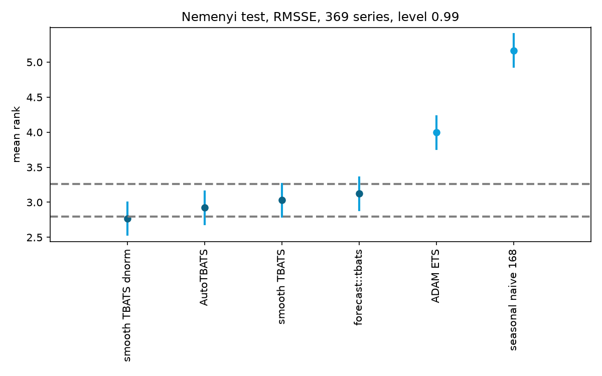
smooth TBATS dnorm against smooth TBATS (distribution "auto") on the 370 series of electricity hourly with rolling-origin evaluation (the windows of run RN13), run once under plan PL8 (lab run RN14). Both are fitted to each window one after the other in the same single-threaded worker, so that their elapsed times are measured under the same load; a failed fit gets the seasonal naive 168 forecasts and no interval. Per series, the RMSSE, the coverage of the 95% interval and the elapsed time averaged over the 7 origins; one-sided t-tests over series on the mean log ratio of RMSSE (auto over dnorm), the mean coverage of dnorm minus 0.95 and the mean log ratio of elapsed time (dnorm over auto), adjusted by Holm over the three; the Nemenyi test on the six methods (A1). Series 322 has an undefined RMSSE and is left out.
Setup: studied smooth TBATS dnorm, smooth TBATS · cases electricity hourly · procedure rolling-origin evaluation · lens RMSSE, relative RMSSE, coverage, elapsed time
- R1 relative RMSSE (geometric mean) = 0.9275 99% confidence interval 0.7825 to 1.0994 (method: smooth TBATS dnorm, comparator: smooth TBATS)
- R2 relative elapsed time (geometric mean) = 0.6368 99% confidence interval 0.619 to 0.6552 (method: smooth TBATS dnorm, comparator: smooth TBATS)
- R3 coverage of smooth TBATS dnorm minus 0.95 (mean) = -0.0168 99% confidence interval -0.0236 to -0.01
- R4 log ratio of RMSSE, smooth TBATS to smooth TBATS dnorm (mean) = 0.0753 99% confidence interval -0.0947 to 0.2453
- R5 log ratio of elapsed time, smooth TBATS dnorm to smooth TBATS (mean) = -0.4512 99% confidence interval -0.4797 to -0.4228
- R6 critical distance, Nemenyi test (RMSSE) = 0.4633 (level: 0.99)
- R7 series in Nemenyi test (count) = 369
- R8 p-value, rmcb test of equal mean ranks (RMSSE) (p_value) = 0.0000
- R9 series excluded by undefined RMSSE (count) = 1
| Row | method | RMSSE (mean) | RMSSE (median) | coverage (nominal level: 0.95) (mean) | elapsed time (median) | series failed (count) | fits failed (count) |
|---|---|---|---|---|---|---|---|
| r1 | smooth TBATS | 0.7948 | 0.6644 | 0.954 | 12.64 | 0 | 0 |
| r2 | smooth TBATS dnorm | 0.7836 | 0.6554 | 0.9332 | 8.031 | 0 | 0 |
| Row | method | mean rank of RMSSE, Nemenyi test (mean) | mean rank of RMSSE, Nemenyi test (bound: 99% interval, lower) | mean rank of RMSSE, Nemenyi test (bound: 99% interval, upper) |
|---|---|---|---|---|
| r1 | smooth TBATS | 3.03 | 2.798 | 3.261 |
| r2 | forecast::tbats | 3.122 | 2.89 | 3.354 |
| r3 | AutoTBATS | 2.921 | 2.69 | 3.153 |
| r4 | ADAM ETS | 3.995 | 3.763 | 4.226 |
| r5 | seasonal naive 168 | 5.165 | 4.934 | 5.397 |
| r6 | smooth TBATS dnorm | 2.767 | 2.535 | 2.999 |
| Row | measure | p-value, one-sided t-test (p_value) | Holm-adjusted p-value, one-sided t-test (p_value) | series in the t-test (count) | series excluded by a non-finite value (count) |
|---|---|---|---|---|---|
| r1 | RMSSE | 0.8738 | 0.8738 | 369 | 0 |
| r2 | coverage | 0.0000 | 0.0000 | 369 | 0 |
| r3 | elapsed time | 0.0000 | 0.0000 | 369 | 0 |
Derivation of the impulse responses of a local level with an ARMA part under ARMA errors and under ADAM's additive ARMA component, and their limits.
Foundation: linear difference equations and power series in the backshift operator $B$ · Assumes: C22
- Under ARMA errors, with stationary gives , with , , and . (definition; from D2, C22)
- The level of the ARMA-errors model moves by , so a unit shock at moves by and by for . (substitution; from S1, D2)
- : the level keeps of every shock, and its increments are autocorrelated unless , that is, unless there is no ARMA part, given that is invertible. (limit; from S1, S2)
- Under ADAM's additive ARMA component, with and , so a unit shock at moves by for . (definition; from D1)
- : the level keeps of every shock, its increments are white noise, and the response of the ARMA part, , decays to zero. (limit; from S1, S4)
- For an AR(1), : , which grows without bound as when , while . (substitution; from S3, S5)
Limitations
The accuracy measure of the M4 hourly tests changed after their results were seen: MASE decided the tests of C4, C5, C6 and C9 (lab run RN8), the guarantor then judged MASE unsuitable and set RMSSE (decision DC4 of the lab record), and C10 to C13 restate those hypotheses on RMSSE and test them on the same M4 test split (run RN11), so they are not independent of C4 to C6 and C9.
The t-tests and their intervals treat the series as independent; the series of one data set share calendar and weather effects, so the intervals may be too narrow.
The electricity evaluation covers one week, the 7 daily origins before 2014-09-08, of the clients of one utility; other weeks or seasons of the year may rank the methods differently.
Elapsed times depend on the machine and on the language: forecast::tbats runs in R and the other methods in Python, the M4 runs ran on a cloud machine and the electricity runs on the guarantor's computer, and each time includes its language's overhead per fit.
The lab record flags plans PL1, PL5 and PL7 with code changed after the plan; between PL1 and its run only m4_hourly.py changed, not the script the run used; between PL5 and its run only electricity_hourly.py was added; between PL7 and its run the change set the null hypothesis of superiority that PL7's design specifies.
References
- https://raw.githubusercontent.com/Mcompetitions/M4-methods/master/Dataset/Train/Hourly-train.csv https://raw.githubusercontent.com/Mcompetitions/M4-methods/master/Dataset/Train/Hourly-train.csv Used by: A5
- https://raw.githubusercontent.com/Mcompetitions/M4-methods/master/Dataset/Test/Hourly-test.csv https://raw.githubusercontent.com/Mcompetitions/M4-methods/master/Dataset/Test/Hourly-test.csv Used by: A6
- https://raw.githubusercontent.com/mbohlkeschneider/gluon-ts/mv_release/datasets/electricity_nips.tar.gz https://raw.githubusercontent.com/mbohlkeschneider/gluon-ts/mv_release/datasets/electricity_nips.tar.gz Used by: A7
- De Livera et al. (2011) De Livera, A. M., Hyndman, R. J., & Snyder, R. D. (2011). Forecasting Time Series With Complex Seasonal Patterns Using Exponential Smoothing. Journal of the American Statistical Association, 106(496), 1513–1527. doi:10.1198/jasa.2011.tm09771 Used by: Context, D2
- Hyndman and Khandakar (2008) Hyndman, R. J., & Khandakar, Y. (2008). Automatic Time Series Forecasting: The forecast Package for R. Journal of Statistical Software, 27(3). doi:10.18637/jss.v027.i03 Used by: D3
- Makridakis et al. (2020) Makridakis, S., Spiliotis, E., & Assimakopoulos, V. (2020). The M4 Competition: 100,000 time series and 61 forecasting methods. International Journal of Forecasting, 36(1), 54–74. doi:10.1016/j.ijforecast.2019.04.014 Used by: D7
- Makridakis et al. (2022) Makridakis, S., Spiliotis, E., & Assimakopoulos, V. (2022). M5 accuracy competition: Results, findings, and conclusions. International Journal of Forecasting, 38(4), 1346–1364. doi:10.1016/j.ijforecast.2021.11.013 Used by: D16
- Svetunkov (2023) Svetunkov, I. (2023). Forecasting and Analytics with the Augmented Dynamic Adaptive Model (ADAM). Chapman and Hall/CRC. doi:10.1201/9781003452652 Used by: Context, D5
- doi:10.24432/C58C86 doi:10.24432/C58C86 Used by: D18
- Hyndman and Koehler (2006) Hyndman, R. J., & Koehler, A. B. (2006). Another look at measures of forecast accuracy. International Journal of Forecasting, 22(4), 679–688. doi:10.1016/j.ijforecast.2006.03.001 Used by: D10
- https://jmlr.org/papers/v7/demsar06a.html https://jmlr.org/papers/v7/demsar06a.html Used by: D15
- https://github.com/Nixtla/statsforecast https://github.com/Nixtla/statsforecast Used by: D4
Artefacts
- A1 · figure · data_plot Nemenyi test on the per-series RMSSE of the six methods on the electricity data (369 series, level 0.99): mean rank of each method with its 99% interval, from run RN14 (smooth TBATS, smooth TBATS dnorm) and run RN13 (the other four). nemenyi_electricity_six_methods.png
- A2 · table CSV written by run RN14 with the per-method values of smooth TBATS and smooth TBATS dnorm (E5.T1), at full precision. dnorm_methods.csv
- A3 · table CSV written by run RN14 with the three t-tests of plan PL8 and the relative RMSSE and elapsed time with their intervals (E5.T3, E5.R1 to E5.R5), at full precision. dnorm_tests.csv
- A4 · table CSV written by run RN14 with the Nemenyi test of the six methods: mean ranks, intervals, critical distance (E5.T2, E5.R6 to E5.R8), at full precision. nemenyi_electricity_six_methods.csv
- A5 · data · https://raw.githubusercontent.com/Mcompetitions/M4-methods/master/Dataset/Train/Hourly-train.csv M4 Hourly-train.csv (text/csv), saved by hand on 2026-11-11; recorded in the lab record as SR1 on 2026-11-11. venue: GitHub, Mcompetitions/M4-methods. Written by others. M4 competition hourly data, train samples, one series per row Published by a third party at the URI; the claimset gives its hash, not the file, and the file keeps its publisher's terms. Hourly-train.csv
- A6 · data · https://raw.githubusercontent.com/Mcompetitions/M4-methods/master/Dataset/Test/Hourly-test.csv M4 Hourly-test.csv (text/csv), saved by hand on 2026-11-11; recorded in the lab record as SR2 on 2026-11-11. venue: GitHub, Mcompetitions/M4-methods. Written by others. M4 competition hourly data, test samples, one series per row Published by a third party at the URI; the claimset gives its hash, not the file, and the file keeps its publisher's terms. Hourly-test.csv
- A7 · data · https://raw.githubusercontent.com/mbohlkeschneider/gluon-ts/mv_release/datasets/electricity_nips.tar.gz GluonTS electricity_nips data set (application/gzip), saved by hand on 2026-11-12; recorded in the lab record as SR3 on 2026-11-12. venue: GitHub, mbohlkeschneider/gluon-ts (branch mv_release). Written by others. Hourly electricity consumption (kW) of 370 clients of a Portuguese utility, from the UCI ElectricityLoadDiagrams20112014 data, as prepared for DeepAR (Salinas et al.): train/data.json ends 2014-09-01 01:00, test/data.json holds 7 daily rolling windows ending 2014-09-02 to 2014-09-08 01:00, in GluonTS JSON lines. Published by a third party at the URI; the claimset gives its hash, not the file, and the file keeps its publisher's terms. electricity_nips.tar.gz
- A8 · data Every result of the lab record (1308 results of 14 runs) at full precision: the lab result's ID, its run, the quantity as the run's script named it, its conditions and its value (both as JSON). The evidence's tables give the values to four significant digits. smooth-tbats.results.csv
- A9 · lab_record Lab record of the study: questions, hypotheses, plans, runs, results and decisions, as an append-only, hash-chained event log (Claimset lab record specification v0.21, begun 2026-11-11; exported with claimset 0.41.6). lab.jsonl
- A10 · code The study's scripts: formulation_checks.py (E1), m4_hourly.py and m4_forecast_tbats.R (E2, E3), electricity_hourly.py (E4) and electricity_dnorm.py (E5), at the last commit of the study's code; each evidence names the commit it ran at. smooth-tbats
Score
Support of the paper: 93, Well supported
Scores are computed by rules from the claimset file (EntryLib rubric 0.4): they check the record, not the science, and may change as the rubric and reviews develop. The rubric. Every issue as text, for an agent preparing the next version.
The mean of its 6 principal claims; the lowest is C10 at 89. Open problems in the principal claims and what they rest on, each counted once, with the most it costs a claim:
- −6 Open problems Limitation L1 (could bias magnitude, not mitigated): The accuracy measure of the M4 hourly tests changed after their results were seen: MASE decided the tests of C4, C5, C6 and C9 (lab run RN8), the guarantor then judged MASE unsuitable and set RMSSE (decision DC4 of the lab record), and C10 to C13 restate those hypotheses on RMSSE and test them on the same M4 test split (run RN11), so they are not independent of C4 to C6 and C9. In C4, C5, C6, C9, C10, C11, C12, C13. To remove it: Mitigate it with evidence, or narrow the claim's scope so that it no longer applies.
- −6 Open problems Limitation L3 (could bias magnitude, not mitigated): The electricity evaluation covers one week, the 7 daily origins before 2014-09-08, of the clients of one utility; other weeks or seasons of the year may rank the methods differently. In C14, C15, C16, C17, C18, C19, C20. To remove it: Mitigate it with evidence, or narrow the claim's scope so that it no longer applies.
- −3 Plan The lab record flags the test: code changed after plan. In C1, C3, C10, C13, C17. To remove it: Rerun the test as planned, or explain the flag in a limitation.
- −1 Open problems Limitation L2 (reduces precision, not mitigated): The t-tests and their intervals treat the series as independent; the series of one data set share calendar and weather effects, so the intervals may be too narrow. In C4, C5, C6, C7, C10, C11, C12, C14, C15, C16, C18, C19, C20. To remove it: Mitigate it with evidence, or narrow the claim's scope so that it no longer applies.
- −3 Open problems Limitation L5 (reduces precision, not mitigated): The lab record flags plans PL1, PL5 and PL7 with code changed after the plan; between PL1 and its run only m4_hourly.py changed, not the script the run used; between PL5 and its run only electricity_hourly.py was added; between PL7 and its run the change set the null hypothesis of superiority that PL7's design specifies. In C1, C2, C3, C10, C11, C12, C13, C14, C15, C16, C17. To remove it: Mitigate it with evidence, or narrow the claim's scope so that it no longer applies.
Claims
C1: 94, Well supported
Novelty: new, by the authors
- −3 Plan The lab record flags the test: code changed after plan. To remove it: Rerun the test as planned, or explain the flag in a limitation.
- −3 Open problems Limitation L5 (reduces precision, not mitigated): The lab record flags plans PL1, PL5 and PL7 with code changed after the plan; between PL1 and its run only m4_hourly.py changed, not the script the run used; between PL5 and its run only electricity_hourly.py was added; between PL7 and its run the change set the null hypothesis of superiority that PL7's design specifies. To remove it: Mitigate it with evidence, or narrow the claim's scope so that it no longer applies.
C2: 97, Well supported
- −3 Open problems Limitation L5 (reduces precision, not mitigated): The lab record flags plans PL1, PL5 and PL7 with code changed after the plan; between PL1 and its run only m4_hourly.py changed, not the script the run used; between PL5 and its run only electricity_hourly.py was added; between PL7 and its run the change set the null hypothesis of superiority that PL7's design specifies. To remove it: Mitigate it with evidence, or narrow the claim's scope so that it no longer applies.
C3: 94, Well supported
Novelty: new, by the authors
- −3 Plan The lab record flags the test: code changed after plan. To remove it: Rerun the test as planned, or explain the flag in a limitation.
- −3 Open problems Limitation L5 (reduces precision, not mitigated): The lab record flags plans PL1, PL5 and PL7 with code changed after the plan; between PL1 and its run only m4_hourly.py changed, not the script the run used; between PL5 and its run only electricity_hourly.py was added; between PL7 and its run the change set the null hypothesis of superiority that PL7's design specifies. To remove it: Mitigate it with evidence, or narrow the claim's scope so that it no longer applies.
C4: 93, Well supported
Novelty: new, by the authors
- −6 Open problems Limitation L1 (could bias magnitude, not mitigated): The accuracy measure of the M4 hourly tests changed after their results were seen: MASE decided the tests of C4, C5, C6 and C9 (lab run RN8), the guarantor then judged MASE unsuitable and set RMSSE (decision DC4 of the lab record), and C10 to C13 restate those hypotheses on RMSSE and test them on the same M4 test split (run RN11), so they are not independent of C4 to C6 and C9. To remove it: Mitigate it with evidence, or narrow the claim's scope so that it no longer applies.
- −1 Open problems Limitation L2 (reduces precision, not mitigated): The t-tests and their intervals treat the series as independent; the series of one data set share calendar and weather effects, so the intervals may be too narrow. To remove it: Mitigate it with evidence, or narrow the claim's scope so that it no longer applies.
C5: 93, Well supported
Novelty: new, by the authors
- −6 Open problems Limitation L1 (could bias magnitude, not mitigated): The accuracy measure of the M4 hourly tests changed after their results were seen: MASE decided the tests of C4, C5, C6 and C9 (lab run RN8), the guarantor then judged MASE unsuitable and set RMSSE (decision DC4 of the lab record), and C10 to C13 restate those hypotheses on RMSSE and test them on the same M4 test split (run RN11), so they are not independent of C4 to C6 and C9. To remove it: Mitigate it with evidence, or narrow the claim's scope so that it no longer applies.
- −1 Open problems Limitation L2 (reduces precision, not mitigated): The t-tests and their intervals treat the series as independent; the series of one data set share calendar and weather effects, so the intervals may be too narrow. To remove it: Mitigate it with evidence, or narrow the claim's scope so that it no longer applies.
C6: 93, Well supported
Novelty: new, by the authors
- −6 Open problems Limitation L1 (could bias magnitude, not mitigated): The accuracy measure of the M4 hourly tests changed after their results were seen: MASE decided the tests of C4, C5, C6 and C9 (lab run RN8), the guarantor then judged MASE unsuitable and set RMSSE (decision DC4 of the lab record), and C10 to C13 restate those hypotheses on RMSSE and test them on the same M4 test split (run RN11), so they are not independent of C4 to C6 and C9. To remove it: Mitigate it with evidence, or narrow the claim's scope so that it no longer applies.
- −1 Open problems Limitation L2 (reduces precision, not mitigated): The t-tests and their intervals treat the series as independent; the series of one data set share calendar and weather effects, so the intervals may be too narrow. To remove it: Mitigate it with evidence, or narrow the claim's scope so that it no longer applies.
C7: 93, Well supported
Novelty: new, by the authors
- −6 Open problems Limitation L4 (could bias magnitude, not mitigated): Elapsed times depend on the machine and on the language: forecast::tbats runs in R and the other methods in Python, the M4 runs ran on a cloud machine and the electricity runs on the guarantor's computer, and each time includes its language's overhead per fit. To remove it: Mitigate it with evidence, or narrow the claim's scope so that it no longer applies.
- −1 Open problems Limitation L2 (reduces precision, not mitigated): The t-tests and their intervals treat the series as independent; the series of one data set share calendar and weather effects, so the intervals may be too narrow. To remove it: Mitigate it with evidence, or narrow the claim's scope so that it no longer applies.
C9: 94, Well supported
Novelty: new, by the authors
- −6 Open problems Limitation L1 (could bias magnitude, not mitigated): The accuracy measure of the M4 hourly tests changed after their results were seen: MASE decided the tests of C4, C5, C6 and C9 (lab run RN8), the guarantor then judged MASE unsuitable and set RMSSE (decision DC4 of the lab record), and C10 to C13 restate those hypotheses on RMSSE and test them on the same M4 test split (run RN11), so they are not independent of C4 to C6 and C9. To remove it: Mitigate it with evidence, or narrow the claim's scope so that it no longer applies.
C10: 89, Well supported
Novelty: new, by the authors
- −6 Open problems Limitation L1 (could bias magnitude, not mitigated): The accuracy measure of the M4 hourly tests changed after their results were seen: MASE decided the tests of C4, C5, C6 and C9 (lab run RN8), the guarantor then judged MASE unsuitable and set RMSSE (decision DC4 of the lab record), and C10 to C13 restate those hypotheses on RMSSE and test them on the same M4 test split (run RN11), so they are not independent of C4 to C6 and C9. To remove it: Mitigate it with evidence, or narrow the claim's scope so that it no longer applies.
- −3 Plan The lab record flags the test: code changed after plan. To remove it: Rerun the test as planned, or explain the flag in a limitation.
- −1 Open problems Limitation L2 (reduces precision, not mitigated): The t-tests and their intervals treat the series as independent; the series of one data set share calendar and weather effects, so the intervals may be too narrow. To remove it: Mitigate it with evidence, or narrow the claim's scope so that it no longer applies.
- −1 Open problems Limitation L5 (reduces precision, not mitigated): The lab record flags plans PL1, PL5 and PL7 with code changed after the plan; between PL1 and its run only m4_hourly.py changed, not the script the run used; between PL5 and its run only electricity_hourly.py was added; between PL7 and its run the change set the null hypothesis of superiority that PL7's design specifies. To remove it: Mitigate it with evidence, or narrow the claim's scope so that it no longer applies.
C11: 92, Well supported
Novelty: new, by the authors
- −6 Open problems Limitation L1 (could bias magnitude, not mitigated): The accuracy measure of the M4 hourly tests changed after their results were seen: MASE decided the tests of C4, C5, C6 and C9 (lab run RN8), the guarantor then judged MASE unsuitable and set RMSSE (decision DC4 of the lab record), and C10 to C13 restate those hypotheses on RMSSE and test them on the same M4 test split (run RN11), so they are not independent of C4 to C6 and C9. To remove it: Mitigate it with evidence, or narrow the claim's scope so that it no longer applies.
- −1 Open problems Limitation L2 (reduces precision, not mitigated): The t-tests and their intervals treat the series as independent; the series of one data set share calendar and weather effects, so the intervals may be too narrow. To remove it: Mitigate it with evidence, or narrow the claim's scope so that it no longer applies.
- −1 Open problems Limitation L5 (reduces precision, not mitigated): The lab record flags plans PL1, PL5 and PL7 with code changed after the plan; between PL1 and its run only m4_hourly.py changed, not the script the run used; between PL5 and its run only electricity_hourly.py was added; between PL7 and its run the change set the null hypothesis of superiority that PL7's design specifies. To remove it: Mitigate it with evidence, or narrow the claim's scope so that it no longer applies.
C12: 92, Well supported
Novelty: new, by the authors
- −6 Open problems Limitation L1 (could bias magnitude, not mitigated): The accuracy measure of the M4 hourly tests changed after their results were seen: MASE decided the tests of C4, C5, C6 and C9 (lab run RN8), the guarantor then judged MASE unsuitable and set RMSSE (decision DC4 of the lab record), and C10 to C13 restate those hypotheses on RMSSE and test them on the same M4 test split (run RN11), so they are not independent of C4 to C6 and C9. To remove it: Mitigate it with evidence, or narrow the claim's scope so that it no longer applies.
- −1 Open problems Limitation L2 (reduces precision, not mitigated): The t-tests and their intervals treat the series as independent; the series of one data set share calendar and weather effects, so the intervals may be too narrow. To remove it: Mitigate it with evidence, or narrow the claim's scope so that it no longer applies.
- −1 Open problems Limitation L5 (reduces precision, not mitigated): The lab record flags plans PL1, PL5 and PL7 with code changed after the plan; between PL1 and its run only m4_hourly.py changed, not the script the run used; between PL5 and its run only electricity_hourly.py was added; between PL7 and its run the change set the null hypothesis of superiority that PL7's design specifies. To remove it: Mitigate it with evidence, or narrow the claim's scope so that it no longer applies.
C13: 90, Well supported
Novelty: new, by the authors
- −6 Open problems Limitation L1 (could bias magnitude, not mitigated): The accuracy measure of the M4 hourly tests changed after their results were seen: MASE decided the tests of C4, C5, C6 and C9 (lab run RN8), the guarantor then judged MASE unsuitable and set RMSSE (decision DC4 of the lab record), and C10 to C13 restate those hypotheses on RMSSE and test them on the same M4 test split (run RN11), so they are not independent of C4 to C6 and C9. To remove it: Mitigate it with evidence, or narrow the claim's scope so that it no longer applies.
- −3 Plan The lab record flags the test: code changed after plan. To remove it: Rerun the test as planned, or explain the flag in a limitation.
- −1 Open problems Limitation L5 (reduces precision, not mitigated): The lab record flags plans PL1, PL5 and PL7 with code changed after the plan; between PL1 and its run only m4_hourly.py changed, not the script the run used; between PL5 and its run only electricity_hourly.py was added; between PL7 and its run the change set the null hypothesis of superiority that PL7's design specifies. To remove it: Mitigate it with evidence, or narrow the claim's scope so that it no longer applies.
C14: 92, Well supported
Novelty: new, by the authors
- −6 Open problems Limitation L3 (could bias magnitude, not mitigated): The electricity evaluation covers one week, the 7 daily origins before 2014-09-08, of the clients of one utility; other weeks or seasons of the year may rank the methods differently. To remove it: Mitigate it with evidence, or narrow the claim's scope so that it no longer applies.
- −1 Open problems Limitation L2 (reduces precision, not mitigated): The t-tests and their intervals treat the series as independent; the series of one data set share calendar and weather effects, so the intervals may be too narrow. To remove it: Mitigate it with evidence, or narrow the claim's scope so that it no longer applies.
- −1 Open problems Limitation L5 (reduces precision, not mitigated): The lab record flags plans PL1, PL5 and PL7 with code changed after the plan; between PL1 and its run only m4_hourly.py changed, not the script the run used; between PL5 and its run only electricity_hourly.py was added; between PL7 and its run the change set the null hypothesis of superiority that PL7's design specifies. To remove it: Mitigate it with evidence, or narrow the claim's scope so that it no longer applies.
C15: 92, Well supported
Novelty: new, by the authors
- −6 Open problems Limitation L3 (could bias magnitude, not mitigated): The electricity evaluation covers one week, the 7 daily origins before 2014-09-08, of the clients of one utility; other weeks or seasons of the year may rank the methods differently. To remove it: Mitigate it with evidence, or narrow the claim's scope so that it no longer applies.
- −1 Open problems Limitation L2 (reduces precision, not mitigated): The t-tests and their intervals treat the series as independent; the series of one data set share calendar and weather effects, so the intervals may be too narrow. To remove it: Mitigate it with evidence, or narrow the claim's scope so that it no longer applies.
- −1 Open problems Limitation L5 (reduces precision, not mitigated): The lab record flags plans PL1, PL5 and PL7 with code changed after the plan; between PL1 and its run only m4_hourly.py changed, not the script the run used; between PL5 and its run only electricity_hourly.py was added; between PL7 and its run the change set the null hypothesis of superiority that PL7's design specifies. To remove it: Mitigate it with evidence, or narrow the claim's scope so that it no longer applies.
C16: 92, Well supported
Novelty: new, by the authors
- −6 Open problems Limitation L3 (could bias magnitude, not mitigated): The electricity evaluation covers one week, the 7 daily origins before 2014-09-08, of the clients of one utility; other weeks or seasons of the year may rank the methods differently. To remove it: Mitigate it with evidence, or narrow the claim's scope so that it no longer applies.
- −1 Open problems Limitation L2 (reduces precision, not mitigated): The t-tests and their intervals treat the series as independent; the series of one data set share calendar and weather effects, so the intervals may be too narrow. To remove it: Mitigate it with evidence, or narrow the claim's scope so that it no longer applies.
- −1 Open problems Limitation L5 (reduces precision, not mitigated): The lab record flags plans PL1, PL5 and PL7 with code changed after the plan; between PL1 and its run only m4_hourly.py changed, not the script the run used; between PL5 and its run only electricity_hourly.py was added; between PL7 and its run the change set the null hypothesis of superiority that PL7's design specifies. To remove it: Mitigate it with evidence, or narrow the claim's scope so that it no longer applies.
C17: 90, Well supported
Novelty: new, by the authors
- −6 Open problems Limitation L3 (could bias magnitude, not mitigated): The electricity evaluation covers one week, the 7 daily origins before 2014-09-08, of the clients of one utility; other weeks or seasons of the year may rank the methods differently. To remove it: Mitigate it with evidence, or narrow the claim's scope so that it no longer applies.
- −3 Plan The lab record flags the test: code changed after plan. To remove it: Rerun the test as planned, or explain the flag in a limitation.
- −1 Open problems Limitation L5 (reduces precision, not mitigated): The lab record flags plans PL1, PL5 and PL7 with code changed after the plan; between PL1 and its run only m4_hourly.py changed, not the script the run used; between PL5 and its run only electricity_hourly.py was added; between PL7 and its run the change set the null hypothesis of superiority that PL7's design specifies. To remove it: Mitigate it with evidence, or narrow the claim's scope so that it no longer applies.
C18: 93, Well supported
Novelty: new, by the authors
- −6 Open problems Limitation L3 (could bias magnitude, not mitigated): The electricity evaluation covers one week, the 7 daily origins before 2014-09-08, of the clients of one utility; other weeks or seasons of the year may rank the methods differently. To remove it: Mitigate it with evidence, or narrow the claim's scope so that it no longer applies.
- −1 Open problems Limitation L2 (reduces precision, not mitigated): The t-tests and their intervals treat the series as independent; the series of one data set share calendar and weather effects, so the intervals may be too narrow. To remove it: Mitigate it with evidence, or narrow the claim's scope so that it no longer applies.
C19: 93, Well supported
Novelty: new, by the authors
- −6 Open problems Limitation L3 (could bias magnitude, not mitigated): The electricity evaluation covers one week, the 7 daily origins before 2014-09-08, of the clients of one utility; other weeks or seasons of the year may rank the methods differently. To remove it: Mitigate it with evidence, or narrow the claim's scope so that it no longer applies.
- −1 Open problems Limitation L2 (reduces precision, not mitigated): The t-tests and their intervals treat the series as independent; the series of one data set share calendar and weather effects, so the intervals may be too narrow. To remove it: Mitigate it with evidence, or narrow the claim's scope so that it no longer applies.
C20: 90, Well supported
Novelty: new, by the authors
- −6 Open problems Limitation L3 (could bias magnitude, not mitigated): The electricity evaluation covers one week, the 7 daily origins before 2014-09-08, of the clients of one utility; other weeks or seasons of the year may rank the methods differently. To remove it: Mitigate it with evidence, or narrow the claim's scope so that it no longer applies.
- −3 Open problems Limitation L4 (could bias magnitude, not mitigated): Elapsed times depend on the machine and on the language: forecast::tbats runs in R and the other methods in Python, the M4 runs ran on a cloud machine and the electricity runs on the guarantor's computer, and each time includes its language's overhead per fit. To remove it: Mitigate it with evidence, or narrow the claim's scope so that it no longer applies.
- −1 Open problems Limitation L2 (reduces precision, not mitigated): The t-tests and their intervals treat the series as independent; the series of one data set share calendar and weather effects, so the intervals may be too narrow. To remove it: Mitigate it with evidence, or narrow the claim's scope so that it no longer applies.
Versions
- Version 2 (this page) · 13 November 2026 at 12:34 UTC · updated
- Version 1 · 13 November 2026 at 12:04 UTC · active
Every version is kept in the public registry (github.com/entrylib/registry).